Field Observations during the Eleventh Microwave Water and Energy Balance Experiment (MicroWEX-11): from April 25, 2012, through December 6, 2012
To view this entire report in PDF format, click here.
1. Introduction
For accurate prediction of weather and near-term climate, root-zone soil moisture is one of the most crucial components driving the surface hydrological processes. Soil moisture in the top meter governs moisture and energy fluxes at the land–atmosphere interface, and it plays a significant role in partitioning of precipitation into runoff and infiltration.
Energy and moisture fluxes at the land surface during growing seasons of agricultural crops can be estimated by coupled Soil-Vegetation-Atmosphere-Transfer and crop growth models. Even though the biophysics of moisture and energy transport and of crop growth and development are well-captured in most current models, the errors in initialization, forcings, and computation accumulate over time and the model estimates of soil moisture in the root zone diverge from reality. Remotely sensed microwave observations can be assimilated in these models to improve root zone soil moisture and crop yield estimates.
The microwave signatures at low frequencies, particularly at 1–2 GHz (L-band) and 4–8 GHz (C-band) are very sensitive to soil moisture in the top few centimeters in most vegetated surfaces. Many studies have been conducted in agricultural areas—such as bare soil, grass, soybean, wheat, pasture, and corn—to understand the relationship between soil moisture and microwave remote sensing. It is important to know how microwave signatures vary with soil moisture, evapotranspiration (ET), and biomass during the growing season for a dynamic agricultural canopy with a significant wet biomass of 4–12 kg/m2.
2. Objectives
The goal of MicroWEX-11 was to conduct a season-long experiment, which incorporated active and passive microwave observations for bare soil, a growing season of elephant grass, and sweet corn. The variety of sensors allowed for further understanding of the land–atmosphere interactions during the growing season, and their effect on observed passive microwave signatures at 6.7 GHz and 1.4 GHz and active microwave signatures at 1.25 GHz. These observations match that of the satellite-based passive microwave radiometers, Advanced Microwave Scanning Radiometer-2 (AMSR-2), and the Soil Moisture and Ocean Salinity (SMOS) mission, respectively, and the recently launched National Aeronautics and Space Administration's Soil Moisture Active Passive (SMAP) mission. Specific objectives of MicroWEX-11 include the following:
-
To acquire simultaneous active and passive data for bare soil, elephant grass, and corn.
-
To collect passive and active microwave and other ancillary data to develop preliminary algorithms to estimate microwave signatures for bare soil, elephant grass, and corn.
-
To evaluate feasibility of soil moisture retrievals using passive microwave data at 6.7 GHz and 1.4 GHz and active microwave data at 1.25 GHz for bare soil, growing elephant grass canopy, and corn.
-
To gain insight in the diurnal variation of the dielectric constant of vegetation.
This report describes the observations conducted during the MicroWEX-11.
3. Field Setup
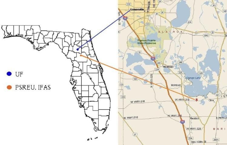
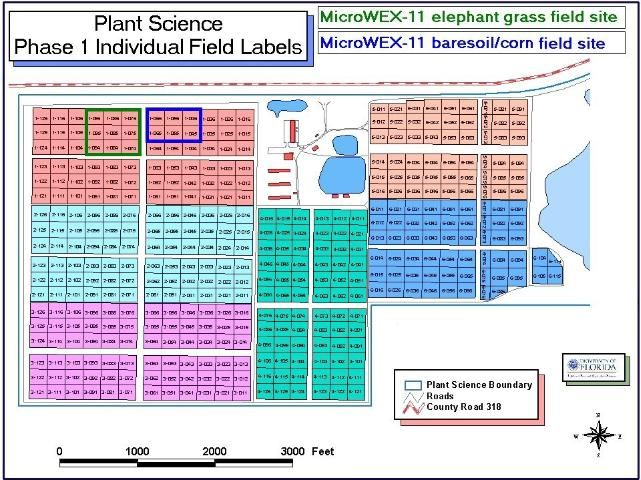
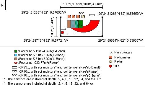
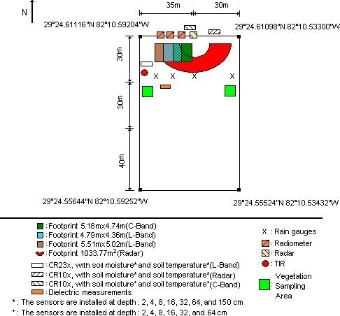
MicroWEX-11 was conducted at the UF/IFAS Extension Plant Science Research and Education Unit (PSREU), Citra, FL. Figures 1 and 2 show the location of the PSREU and the study site for the MicroWEX-11, respectively. The study site was located at the west side of the PSREU (29.4°N, 82.17°W). The instruments consisted of three ground-based microwave radiometer systems, a ground-based microwave radar system, and micrometeorological stations. The ground-based microwave radiometer systems were installed at the location shown in Figure 3(a–c), facing south to avoid the radiometer shadow interfering with the field of view. The ground-based microwave radar system was installed adjacent to the radiometer with a portion of the radar footprint overlapping the radiometer footprint, facing in the same direction as the radiometer system.
The dimensions of the bare soil study site were 65 m × 30 m with the corners of the field located at 29.4102°N 82.1763°W; 29.4102°N 82.1756°W; 29.4099°N 82.1756°W; 29.4100°N 82.1763°W. A linear move system was used for irrigation. The ground-based microwave radiometer and radar systems installation began on May 1 (Day of Year [DoY] 122) in 2012 with micrometeorological stations on DoY 123. (See Table B-1 for corresponding months and dates to the DoY mentioned in this document.) Three micrometeorological stations with soil moisture and soil temperature sensors were installed at the locations shown in Figure 3(a). On DoY 145, the soil moisture and soil temperature sensors were removed to conduct a seedless planting to simulate the roughness of a typical agricultural field during planting, and reburied on DoY 146. Rain gauges were installed on the south edge of the field in line with the outer edge of the UF L-band radiometer footprint and the UF L-band radar footprint. A thermal infrared sensor was installed south of the L-band station.
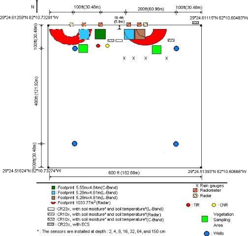
The dimensions of the elephant grass study site were 183 m × 183 m with the corners of the field located at 29.410°N 82.179°W; 29.410°N 82.177°W; 29.409°N 82.177°W; 29.409°N 82.179°W. The elephant grass (Pennisetum purpureum)—of varieties Merkeron, N-13, N-43, and N-51—was in its third year of growth. The row spacing was 182.9 cm (72 inches). A linear move system was used for irrigation. The ground-based microwave radiometer and radar systems installation began on DoY 165 with micrometeorological stations on DoY 170. Three micrometeorological stations with soil moisture and soil temperature sensors were installed at the locations shown in Figure 3(b). Rain gauges were installed south of the radar footprint in line with the outer edge of the UF L-band radiometer footprint and the UF L-band radar footprint. A relative humidity (RH) and temperature sensor were installed at the L-band station. A net radiometer and thermal infrared sensor were installed south of the C-band radiometer. On DoY 185, thermistors were installed to measure canopy temperature.
The dimensions of the corn study site were 100 m × 65 m with the corners of the field located at 29.4102°N 82.1765°W; 29.4102°N 82.1756°W; 29.4093°N 82.1765°W; 29.4093°N 82.1756°W. The corn of variety Yellow Supersweet Hybrid (SH2) Saturn was planted on DoY 230, at an orientation 0º from the east. The plant spacing was 18.4 cm (7 ¼ inches) and the row spacing was 91.4 cm (36 inches). A linear move system was used for irrigation. The ground-based microwave radiometer and radar systems installation began on DoY 227 with micrometeorological stations on DoY 233. Rain gauges were installed south of the radar footprint in line with the outer edge of the UF L-band radiometer footprint and the UF L-band radar footprint. Two micrometeorological stations with soil moisture and soil temperature sensors were installed at the locations shown in Figure 3(c). A thermal infrared sensor was installed south of the L-band station. Starting on DoY 282, dielectric measurements of the vegetation were taken. This report provides detailed information regarding sensors deployed and data collected during the MicroWEX-11.
Credit: http://plantscienceunit.ifas.ufl.edu/directions.shtml
Credit: http://plantscienceunit.ifas.ufl.edu/images/location/p1.jpg
4. Sensors
MicroWEX-11 had six major types of instrument subsystems: (1) the ground-based University of Florida C-band and L-band radiometers, (2) the ground-based University of Michigan L-band radiometer, (3) the ground-based University of Florida L-band radar, (4) the dielectric measurements, (5) the micrometeorological, and (6) the soil subsystem.
4.1 University of Florida Microwave Radiometer Systems
4.1.1 University of Florida C-band Microwave Radiometer (UFCMR)
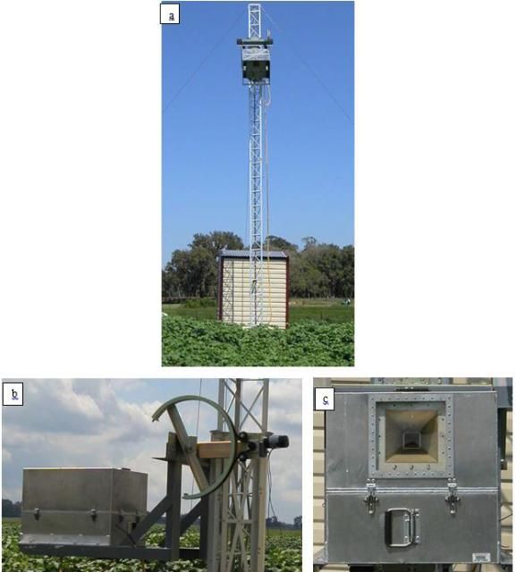
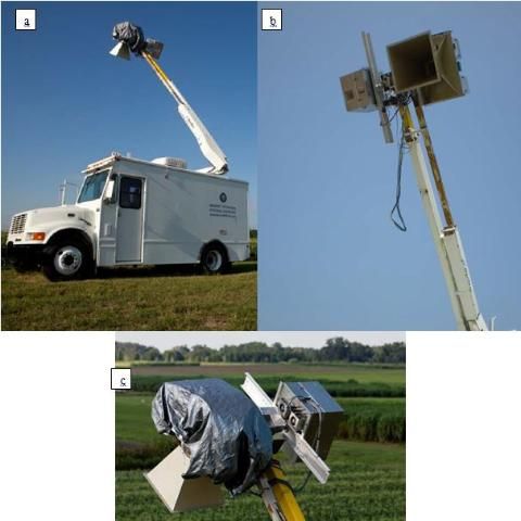
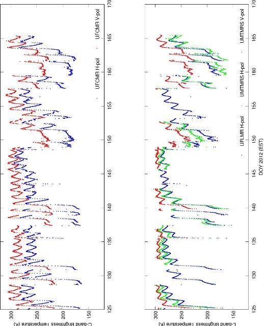
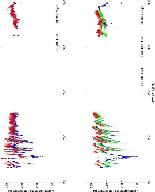
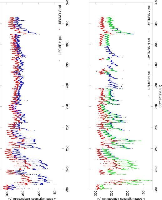
Microwave brightness temperatures at 6.7 GHz (λ = 4.48 cm) were measured every 15 minutes using the University of Florida's C-band Microwave Radiometer system (UFCMR) (Figure 4[a]). The radiometer system consisted of a dual polarization total power radiometer operating at the center frequency of 6.7 GHz housed atop a 10 m tower installed on a 16' trailer bed. The UFCMR was designed and built by the Microwave Geophysics Group at the University of Michigan. It operates at the center frequency at 6.7 GHz, which is near one of the center frequencies on the space-borne AMSR-2 aboard the Japan Aerospace Exploration Agency's Global Change Observation Mission-Water satellite. The UFCMR observed the 5.11 m × 4.67 m, 5.55 m × 4.84 m, and 5.18 m × 4.74 m footprint from a height of 7.15 m, 7.40 m, and 7.25 m for bare soil, elephant grass, and corn, respectively. A rotary system was used to rotate the look-angle of the UFCMR both for field observations and sky measurements. The brightness temperatures were observed at an incidence angle of 40°. The radiometer was calibrated at least once every week with a microwave absorber as warm load and measurement of sky as cold load. Figure 4(b) shows the close-up of the rotary system and 4(c) shows a close-up of the UFCMR antenna. Table 1 lists the UFCMR specifications. Figure A-1–A-3 shows the V- and H-pol brightness temperatures observed at C-band during MicroWEX-11 for the bare soil, elephant grass, and corn field.
Credit: J. Casanova, UF/IFAS
4.1.1.1 Theory of Operation
The UFCMR uses a thermoelectric cooler (TEC) for thermal control of the Radio Frequency (RF) stages for the UFCMR. This is accomplished by the Oven Industries "McShane" thermal controller. McShane is used to cool or heat by Proportional-Integral-Derivative (PID) algorithm with a high degree of precision at 0.01°C. The RF components are all attached to an aluminum plate that must have sufficient thermal mass to eliminate short-term thermal drifts. All components attached to this thermal plate,
The majority of the gain in the system is provided by a gain and filtering block designed by the University of Michigan for the STAR-Light instrument (De Roo 2003). The main advantage of this gain block is the close proximity of all the amplifiers, simplifying the task of thermal control. This gain block was designed for a radiometer working at the radio astronomy window of 1400–1427 MHz, and so the receiver is a heterodyne type with downconversion from the C-band RF to L-band. To minimize the receiver noise figure, a C-band low-noise amplifier (LNA) is used just prior to downconversion. To protect the amplifier from saturation due to out-of-band interference, a relatively wide bandwidth (but low insertion loss) bandpass filter is used just prior to the amplifier. Three components are between the filter and the antenna: a switch for choosing polarization, a switch for monitoring a reference load, and an isolator to minimize changes in the apparent system gain due to differences in the reflections looking upstream from the LNA.
The electrical penetrations use commercially available weatherproof bulkhead connections (Deutsch connectors or equivalent). The heat sinks have been carefully located employing RTV (silicone sealant) to seal the bolt holes. The radome uses 15 mil polycarbonate for radiometric signal penetration. It is sealed to the case using a rubber gasket held down by a square retainer.
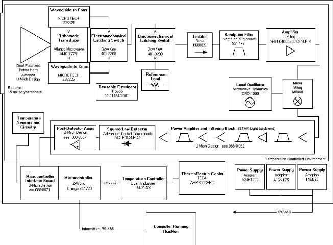
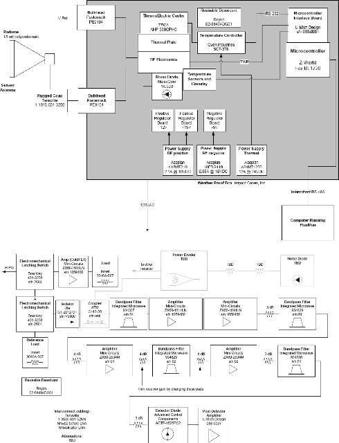
The first SubMiniature version A (SMA) connection is an electromechanical latching, driven by the Z-World control board switches between V- and H-polarization sequentially. The SMA second latching that switches between the analog signal from the first switch and the reference load signal from a reference load resistor sends the analog signal to an isolator, where the signals within 6.4–7.2 GHz in radiofrequency are isolated. Then the central frequency is picked up by a 6.7 GHz bandpass filter, which also protects the amplifier from saturation. A low-noise amplifier (LNA) is used to eliminate the noise figure and adjust gain. A mixer takes the input from the LNA and a local oscillator to output a 1.4 GHz signal to STAR-Light. After the power amplifier and filtering block (Star-Light back-end), the signal is passed through a square law detector and a post-detection amplifier (PDA). The UFCMR is equipped with a microcontroller that is responsible for taking measurements, monitoring the thermal environment, and storing data until a download is requested. A laptop computer is used for running the user interface named FluxMon to communicate with the radiometer through Radiometer Control Language (RadiCL). The radiometer is configured to maintain a particular thermal set point, and make periodic measurements of the brightness at both polarizations sequentially and the reference load. The data collected by the radiometer are not calibrated within the instrument, since calibration errors could corrupt an otherwise useful dataset. Figure 5 shows the block diagram of the UFCMR.
Credit: De Roo (2002)
4.1.2 University of Florida L-Band Microwave Radiometer (UFLMR)
Microwave brightness temperatures at 1.4 GHz (λ = 21.0 cm) were measured every 15 minutes using the University of Florida's L-band Microwave Radiometer system (UFLMR) (Figure 6[a]). The radiometer system consisted of a horizontally polarized total power radiometer operating at the center frequency of 1.4 GHz housed atop a 9.14 m tower installed on a 16' trailer bed. The UFLMR was designed and built by the Microwave Geophysics Group at the University of Michigan. It operates at the center frequency at 1.4 GHz, which is identical to the center frequency on the space-borne SMOS mission. The UFLMR observed the 5.51 m × 5.02 m, 5.28 m × 4.81 m, and 4.79 m × 4.36 m footprint from a height of 7.9 m, 7.76 m, and 6.87 m for bare soil, elephant grass, and corn, respectively. The brightness temperatures were observed at an incidence angle of 40°. A rotary system was used to rotate the look-angle of the UFLMR for both field observations and sky measurements. The radiometer was calibrated at least every week with a measurement of sky as cold load. Figure 6(b) shows a close up of the rotary system and Figure 6(c) shows the antenna of the UFLMR. Table 2 lists the UFLMR specifications. Figure A-1–A-3 shows the horizontally polarized brightness temperatures observed by the UFLMR during MicroWEX-11 for the bare soil, elephant grass, and corn field.
Credit: J. Casanova, UF/IFAS
4.1.2.1 Theory of Operation
The UFLMR is similar to the UFCMR in many respects, using a thermoelectric cooler (TEC) for thermal control, a similar electromechanical switching mechanism, and a Z-World controller. The PDA is the same, and the software is a newer version of RadiCL. The RF block is designed for V- and H-pol switching. However, only the H-pol signal is guided from antenna to coax to the RF block, and the V-pol input to the RF block is a cold load (ColdFet).
In the RF block, the first switch alternates between V- and H-pol and the second alternates between the reference load and the signal from the first switch. An isolator prevents reflections of the input signal. After the isolator, the signal goes through a bandpass filter and then an LNA, followed by a series of bandpass filters and power amplifiers before the square law detector and the PDA. The microcontroller logs voltage and physical temperature measurements. Figure 7 shows the block diagram of the UFLMR.
Credit: De Roo (2010)
4.2 University of Michigan Radiometer
4.2.1 Truck Mounted Radiometer System - L-band (TMRS-L)
The Truck Mounted Radiometer System (TMRS) is a dual-polarized, multi-frequency radiometer system from the University of Michigan that measures microwave brightness temperatures. The radiometer system consisted of a dual polarization total power radiometer housed atop a bucket truck. In this experiment, only the L-band radiometer, operating at the center frequency of 1.4 GHz (λ = 21.0 cm), was used to measure every-15-minute data (Figure 8[a]) in the corn field. The TMRS was designed and built by the Microwave Geophysics Group at the University of Michigan. The height, incident angle, and footprint were identical to the UFLMR. A rotary system was used to rotate the look angle of the TMRS both for field observations and sky measurements. The radiometer was calibrated at least every week with a measurement of sky as cold load. Figure 8(b) shows the antenna and Figure 8(c) shows the close-up of the rotary system of the TMRS-L. Table 3 lists the specifications of the TMRS-L. Figure A-1–A-3 shows the V- and H-pol brightness temperatures observed by the TMRS-L during MicroWEX-11 for the bare soil, elephant grass, and corn field.
Credit: D. Preston, UF/IFAS
4.2.1.1 Theory of Operation
The TMRS-L is similar to the UFLMR and UFCMR in many respects, using a thermoelectric cooler (TEC) for thermal control, a similar electromechanical switching mechanism and a Z-World controller; the PDA is the same, and the software is an older version of RadiCL. The RF block is designed for V- and H-pol switching similar to the UFCMR.
In the RF block, the first switch alternates between V- and H-pol and the second alternates between the reference load and the signal from the first switch. An isolator prevents reflections of the input signal. After the isolator, the signal goes through a bandpass filter and then an LNA, followed by a series of bandpass filters and power amplifiers before the square law detector and the PDA. The microcontroller logs voltage and physical temperature measurements.
4.3 University of Florida Radar System
4.3.1 University of Florida L-band Automated Radar System (UF-LARS)
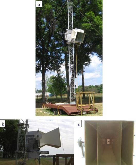
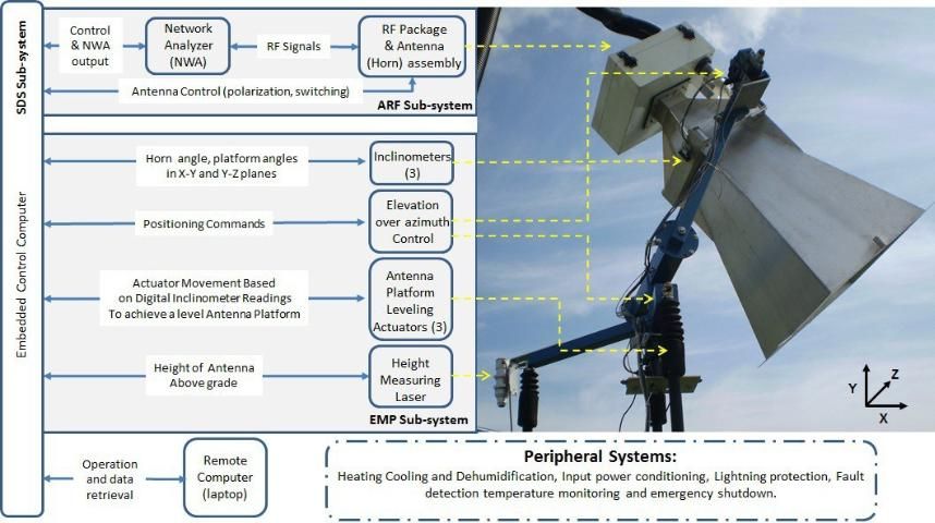
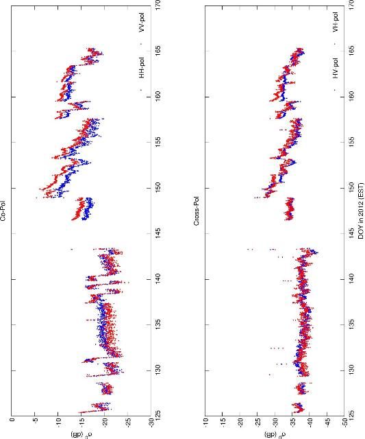
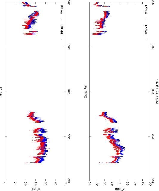
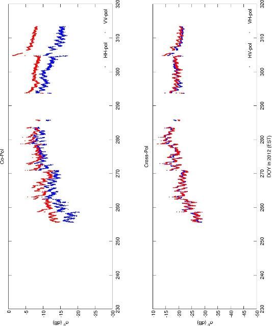
Observations of radar backscatter (σ0) at four polarization combinations, (HH, VV, HV, and VH) and an azimuth range of 0° to 180° with an azimuthal resolution of 9° every 15 minutes resulting in 21 spatial samples were collected using the University of Florida L-band Automated Radar System (UF-LARS) (Figure 9). The UF-LARS is mounted on a 25 m Genie manlift and is comprised of three major sub-systems: (1) the antenna and the RF (ARF) sub-system, (2) the electro-mechanical positioning (EMP) sub-system, and (3) the software control and data acquisition (SDA) sub-system. Figure 10 shows a simplified block diagram of the UF-LARS. The RF subsystem was based upon the established designs for ground-based scatterometers employing a vector network analyzer with simultaneous acquisition of V- and H- polarized returns. These components operate at a center frequency of 1.25 GHz, with a bandwidth of 300 MHz and the one-way 3 dB beamwidth of 14.7° in the E-plane and 19.7° in the H-plane. The polarization isolation at the center frequency was > 37 dB for all principal planes and decreases to about 23 dB at the band edge of 1400 MHz. The EMP sub-system employs an embedded computer and is composed of three digital inclinometers, an elevation-over-azimuth controller, linear actuators, and a laser range finder. The elevation-over-azimuth controller was used to rotate the look-angle of the UF-LARS for both field observations and sky measurements. The antenna incidence angle was set to 40°, while the height was at 16.2 m giving a footprint of an arc, which has a footprint size of 1033.77 m2 based upon the 6 dB beamwidth. The SDA enabled system integration and automated data acquisition using a software control system designed in the Visual C++ environment. Radar calibration included sky measurements, a trihedral corner-reflector (Figure 9), and pole throughout the season. Table 4 summarizes the system specifications. More information regarding the UF-LARS can be found in Nagarajan et al. (2014). Figure A-4–A-6 shows the co-pol and cross-pol radar backscatter observed by the UF-LARS during MicroWEX-11 for the bare soil, elephant grass, and corn field, respectively.
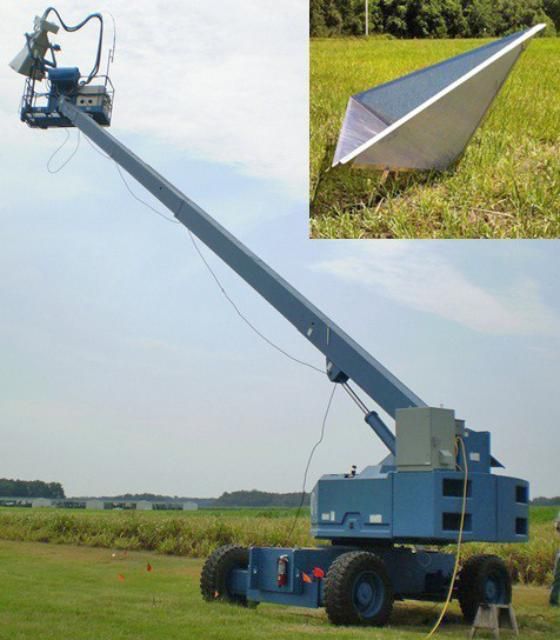
Credit: Nagarajan et al. (2014)
Credit: Nagarajan et al. (2014)
4.4 Dielectric Properties
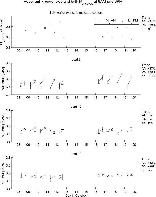
Using a microstrip line sensor, in-vivo dielectric property measurements were conducted on three maize leaves (leaf 8, 10, and 12) from October 8 (DoY 282) to October 19 (DoY 293). An electromagnetic wave is transmitted through a microstrip line resonator. The dielectric constant of the measured sample will modify the capacitance between the stripline and the ground plane, which changes the resonant frequency and the reflectivity of the stripline. Therefore, the change in resonant frequency of the sensor can be used to monitor changes in leaf dielectric properties. To obtain the most accurate results, the microstrip resonator was placed horizontally. Most leaves do not have a perfectly flat surface; so when a leaf is just placed on the sensor, the possibility exists that only an air bubble is measured. To prevent this, the leaf was placed between two Teflon blocks with a thickness of 1 cm. This created a layered measurement setup with a block of Teflon, the sensor, the leaf, and another block of Teflon. Also, Teflon has known constant dielectric properties, making the experiment more reproducible. The measurement setup is presented in Figure 11. All measurements were conducted using a ZVH8 Cable and Antenna Analyzer (ZVH8, 100 kHz to 8 GHz, Rohde & Schwarz, Munich, Germany) with the K42 Vector network Analysis (VNA) and K40 Remote Control option. The VNA sends out the electromagnetic wave to the microstrip line and measures the reflected signal (Van Emmerik 2013).
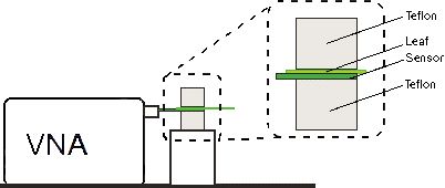
Credit: Van Emmerik (2013)
Measurements were performed manually. Each measurement registered the magnitude [dB] and phase [°] of the reflection coefficient S11 at 1201 points between 2.1 and 4.1 GHz. From DoY 282–293, dielectric measurements were done at 6 a.m. and 6 p.m. corresponding to SMAP measurements. For all dielectric measurements, the following procedure was used. For every leaf, seven measurements were taken. First, a measurement of the Teflon block only was taken. This was done to be able to check the background noise and consistency of the measurements in time, since Teflon should yield the same results. Five measurements were taken on the leaf. Three were taken along the middle nerve of the leaf, at the collar, in the middle of the leaf, and at the tip of the leaf. In the middle of the leaf, two more measurements were taken, one on each side of the blade. Finally, a measurement was taken of air only. Figure 12 illustrates the measurement points on the leaves. Measurements were taken perpendicular at 90° and at 45° to the leaf. Figure A-7 shows the averaged resonant frequency at leaf 8, 10, and 12, including error bars that represent 1 standard deviation. The mean and standard deviation were determined with all 10 measurements (five locations, two angles).
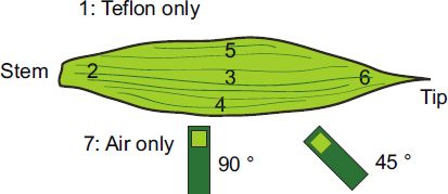
Credit: Van Emmerik (2013)
4.5 Net Radiometer
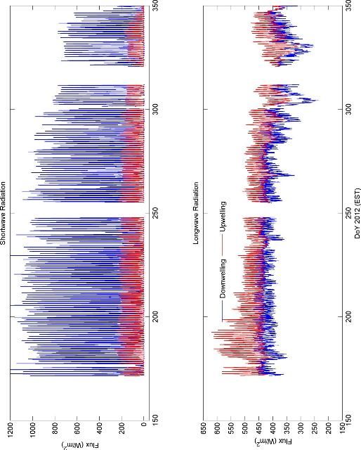
A Kipp and Zonen CNR-1 four-component net radiometer (Figure 13) was located in the elephant grass field, south of the C-band radiometer (as shown in Figure 3[b]), to measure up- and down-welling shortwave and longwave infrared radiation. The sensor consists of two pyranometers (CM-3) and two pyrgeometers (CG-3). The sensor was installed in the elephant grass field, south of the C-band radiometer, at the height of 2.95 m above ground and facing south on DoY 170. On DoY 226, the sensor was moved to a height of 4.8 m to stay above the plant canopy. Table 5 shows the list of specifications of the CNR-1 net radiometer. Figure A-8 shows the down- and up-welling solar (shortwave) and far infrared (longwave) radiation observed during MicroWEX-11.
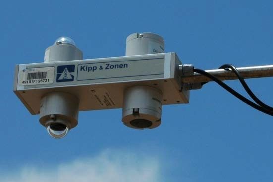
Credit: J. Casanova, UF/IFAS
4.6 Air Temperature and Relative Humidity
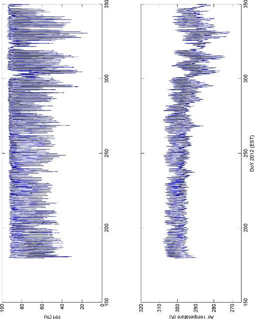
Air temperature and relative humidity were measured every five minutes at the L-band station in the elephant grass field using a Campbell Scientific HMP45C Temperature and Relative Humidity Probe (Campbell Scientific 2006b). Figure A-9 shows the relative humidity and air temperature observations during MicroWEX-11.
4.7 Temperature in the Canopy
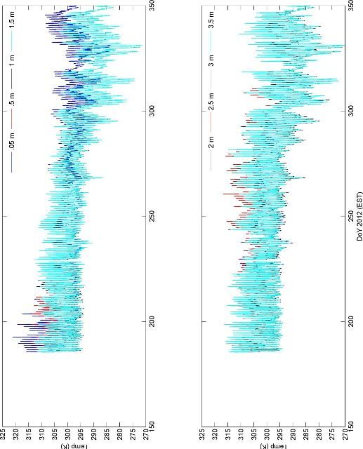
Starting on DoY 185, air temperature, from a height of 0 m to 4.0 m at increments of 0.5 m within the elephant grass canopy, was measured every five minutes west of the C-band station using thermistors on a tripod with an attached PVC pipe, as shown in Figure 14. Figure A-10 shows the canopy temperature observations during MicroWEX-11.
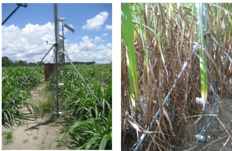
Credit: D. Preston, UF/IFAS
4.8 Thermal Infrared Sensor
Two Apogee instruments IRR-PN thermal infrared sensors were installed during MicroWEX-11: one in the elephant grass and the other in the corn field site. Table 6 shows the list of specifications of the thermal infrared sensors.
4.8.1 Thermal Infrared Sensor (Bare Soil)
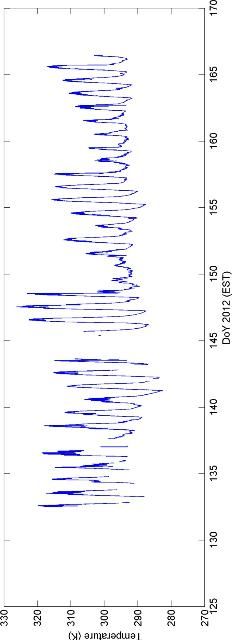
The sensor was installed south of the L-band station (as shown in Figure 3[a]) at a height of 2.14 m to observe skin temperature at nadir. Figure A-11 shows the surface thermal infrared temperature observed during MicroWEX-11.
4.8.2 Thermal Infrared Sensor (Elephant Grass)
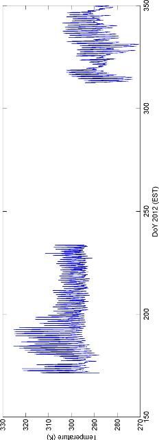
The sensor was installed south of the C-band radiometer (as shown in Figure 3[b]) at a height of 2.5 m to observe skin temperature at nadir. On DoY 223, the sensor was raised to 4.8 m. Figure A-12 shows the thermal infrared temperatures observed during MicroWEX-11.
4.8.3 Thermal Infrared Sensor (Sweet Corn)
The sensor was installed south of the L-band station (as shown in Figure 3[c]) at a height of 2.25 m to observe skin temperature at nadir. Figure A-13 shows the surface thermal infrared temperature observed during MicroWEX-11.
4.9 Soil Temperature Probes
Lab-made temperature probes, based on Campbell Scientific 107-l temperature sensor, were used to measure soil temperature.
4.9.1 Soil Temperature Probes (Bare Soil)
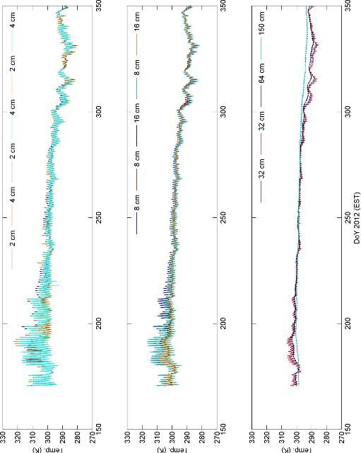
Forty-one temperature probes were placed at depths of 2, 4, 8, 16, 32, 64, and 150 cm measuring every five minutes. At the radar and L-band stations, the depths included two replicate at 2, 4, and 8 cm and one replicate at 16 and 32 cm. The C-band station included one replicate at 2, 4, 8, 16, and 32 cm and did not include a probe at 150 cm. Figure A-14– A-16 shows the soil temperatures observed at the L-band, C-band, and radar station, respectively, during MicroWEX- 11.
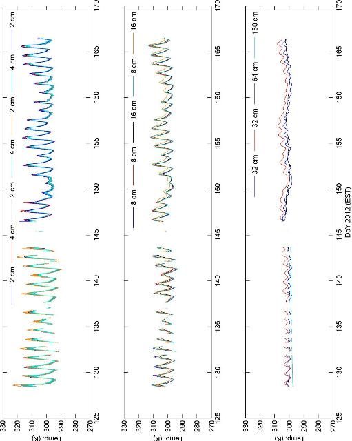
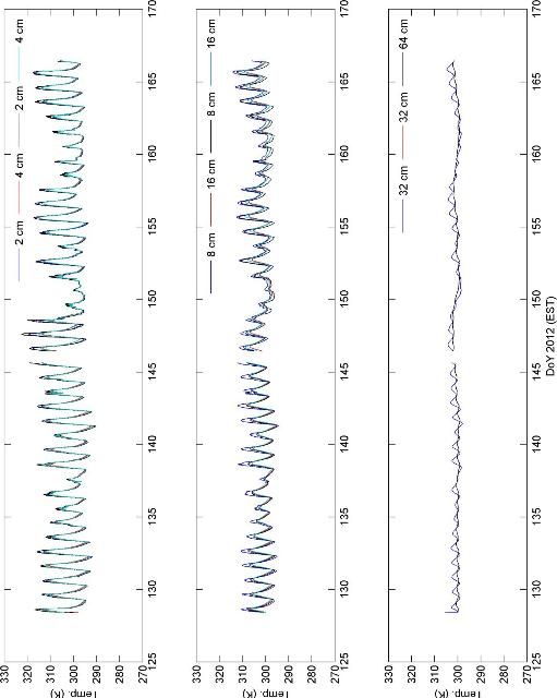
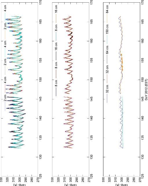
4.9.2 Soil Temperature Probes (Elephant Grass)
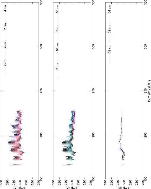
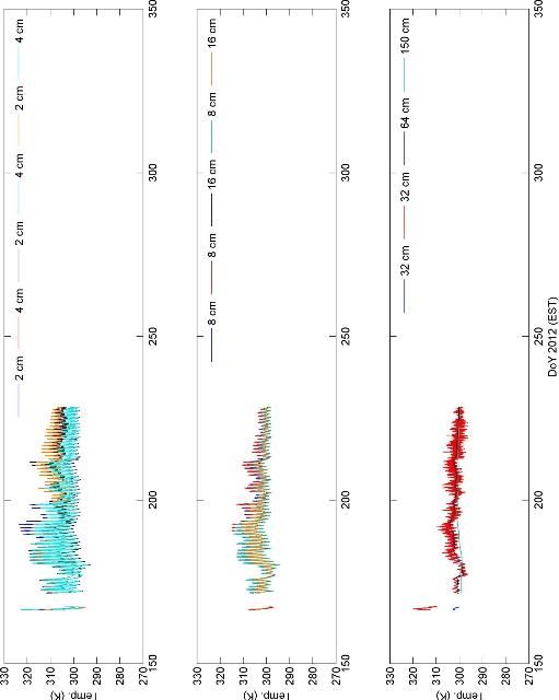
Forty-one temperature probes were placed at depths of 2, 4, 8, 16, 32, 64, and 150 cm measuring every five minutes. At the radar and L-band stations, the depths included two replicate at 2, 4, and 8 cm and one replicate at 16 and 32 cm. The C-band station included one replicate at 2, 4, 8, 16, and 32 cm and did not include a probe at 150 cm. Figure A-17– A-19 shows the soil temperatures observed at the L-band, C-band, and radar station, respectively during MicroWEX- 11.
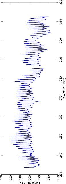
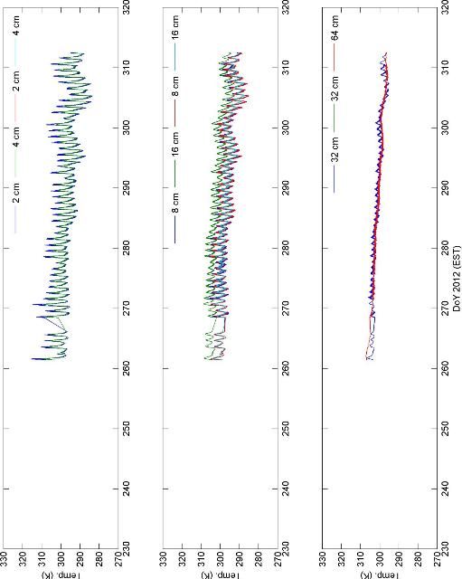
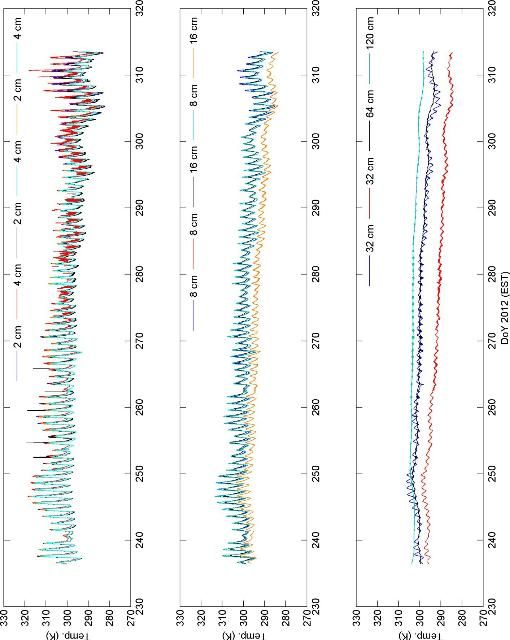
4.9.3 Soil Temperature Probes (Sweet Corn)
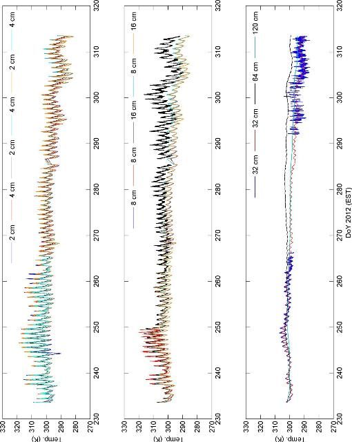
Forty-one temperature probes were placed at depths of 2, 4, 8, 16, 32, 64, and 120 cm measuring every five minutes. At the radar and L-band stations, the depths included two replicate at 2, 4, and 8 cm and one replicate at 16 and 32 cm. The C-band station included one replicate at 2, 4, 8, 16, and 32 cm and did not include a probe at 120 cm. Figure A-20– A-22 shows the soil temperatures observed at the L-band, C-band, and radar station, respectively during MicroWEX- 11.
4.10 Soil Moisture Probes
Campbell Scientific time-domain water content reflectometers (CS616) were used to measure soil volumetric water content. The calibration coefficients were obtained from laboratory calibration and are listed in Table 7.
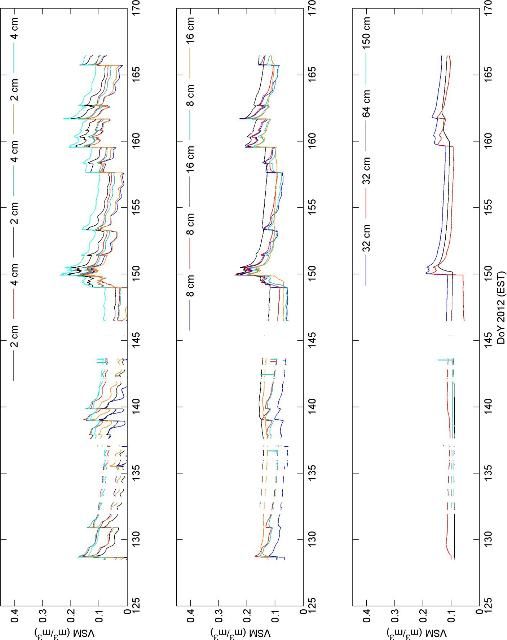
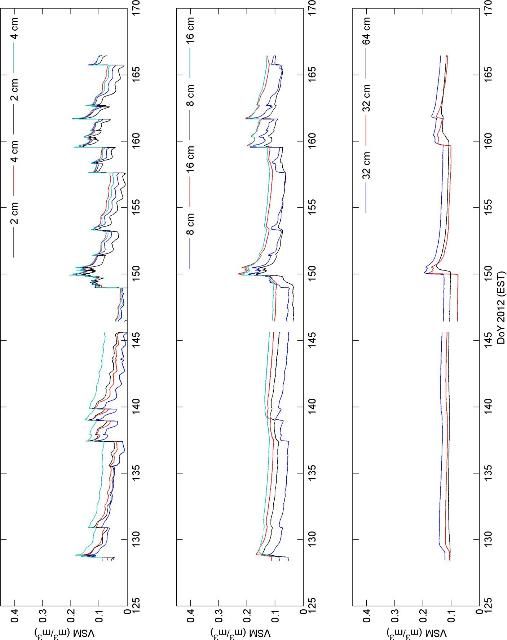
4.10.1 Soil Moisture Probes (Bare Soil)
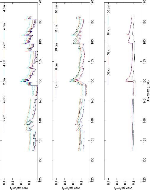
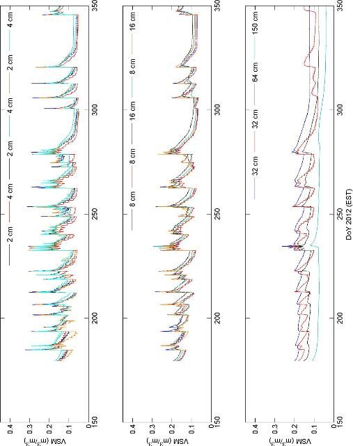
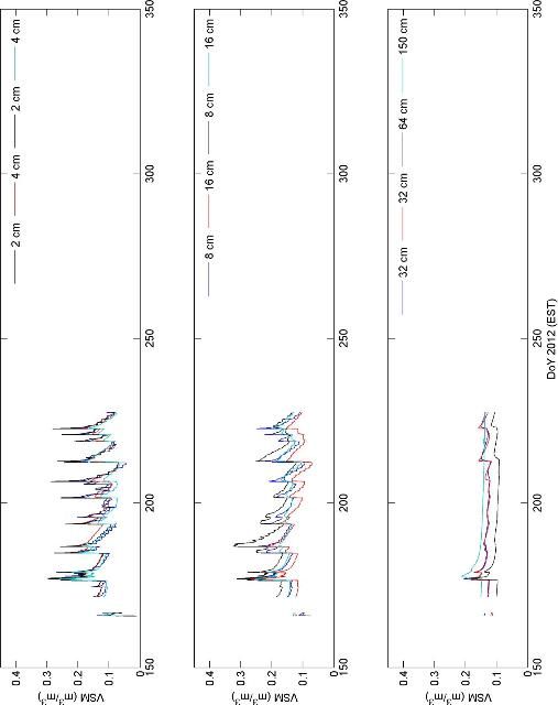
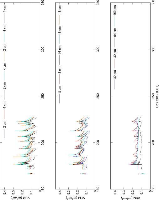
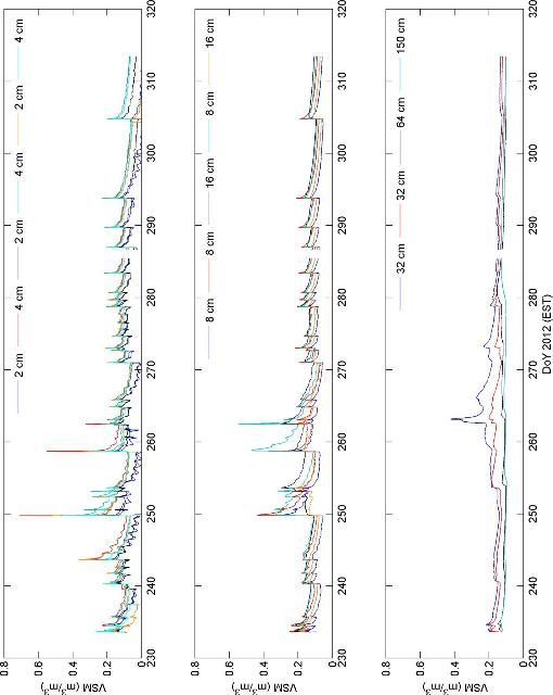
Forty-one reflectometers were placed at depths of 2, 4, 8, 16, 32, 64, and 150 cm measuring every five minutes. At the radar and L-band stations, the depths included two replicate at 2, 4, and 8 cm and one replicate at 16 and 32 cm. The C-band station included one replicate at 2, 4, 8, 16, and 32 cm and did not include a probe at 150 cm. Figure A-23–A-25 shows the volumetric soil moisture contents observed at the L-band, C-band, and radar station, respectively during MicroWEX-11.
4.10.2 Soil Moisture Probes (Elephant Grass)
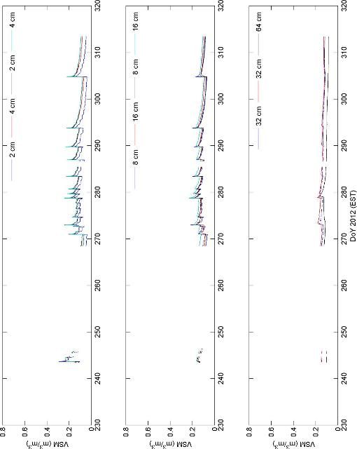
Forty-one reflectometers were placed at depths of 2, 4, 8, 16, 32, 64, and 150 cm measuring every five minutes. For all three stations—radar, C-band, and L-band—the depths included two replicate at 2, 4, and 8 cm and one replicate at 16 and 32 cm. Figure A-26–A-28 shows the volumetric soil moisture contents observed at the L-band, C-band, and radar station, respectively during MicroWEX-11.
4.10.3 Soil Moisture Probes (Sweet Corn)
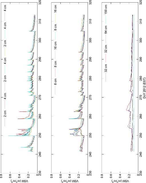
Forty-one reflectometers were placed at depths of 2, 4, 8, 16, 32, 64, and 120 cm measuring every five minutes. At the radar and L-band stations, the depths included two replicate at 2, 4, and 8 cm and one replicate at 16 and 32 cm. The C-band station included one replicate at 2, 4, 8, 16, and 32 cm and did not include a probe at 120 cm. Figure A-29–A-31 shows the volumetric soil moisture contents observed at the L-band, C-band, and radar station, respectively during MicroWEX-11.
4.11 Soil Moisture
Soil moisture measurements using a Dynamax TH2O Soil Moisture Meter were taken on DoY 226 in the elephant grass field. Due to heterogeneity of the elephant grass the UFLARS and the UFLMR were moved to the west side of the field. Multiple measurements were taken from the previous radar and radiometer footprints and the current footprints (Figure 3[b]). The averages and standard deviations of the measurements are shown in Table 8.
4.12 Precipitation
Precipitation and overhead irrigation was determined using six tipping-bucket rain gauges with locations shown in Figure 3(a–c).
4.12.1 Precipitation (Bare Soil)
Four tipping-bucket rain gauges, in line with the outer edge of the UFLMR footprint and at the outer edge of the UFLARS footprint were installed on DoY 128 at a height of 20 cm. Figure A-32 shows the observed precipitation.
4.12.2 Precipitation (Elephant Grass)
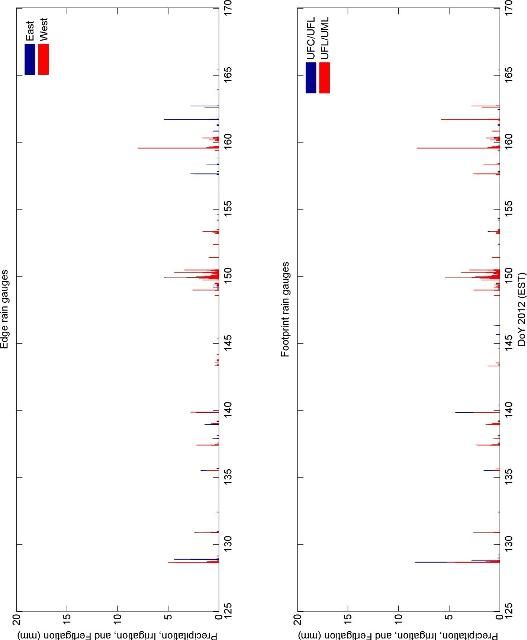
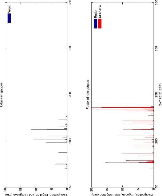
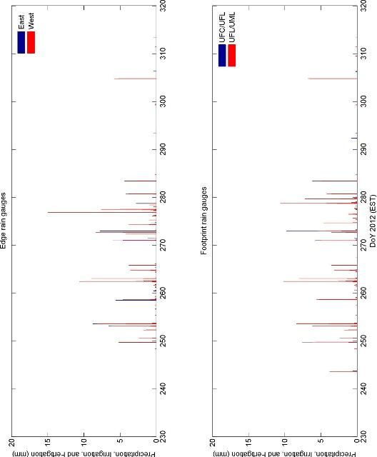
Two tipping-bucket rain gauges in line with the outer edge of the UFLMR footprint were installed on DoY 175 at a height of 20 cm above the ground to catch both precipitation and irrigation. Figure A-33 shows the observed precipitation and overhead irrigation.
4.12.3 Precipitation (Sweet Corn)
Four tipping-bucket rain gauges, two in line with the outer edge of the UFLMR footprint at a height of 3 m above the ground to stay above the height of the corn canopy and two in line with the outer edge of the UFLARS footprint at a height of 20 cm, were installed on DoY 243. Figure A-34 shows the observed precipitation.
5. Vegetation Sampling at the Elephant Grass Site
Vegetation properties in the sampling location, as shown in Figure 3(b), were measured weekly from DoY 201 until DoY 227 with a final sampling on DoY 335 during the field experiment. A vegetation sampling consisted of measurements of clump height and width, as well as biomass. Each sampling included one row of elephant grass in the sampling location. The sampling length started between two clumps and ended at the next midpoint between clumps that was greater than or equal to 4 m from the starting point.
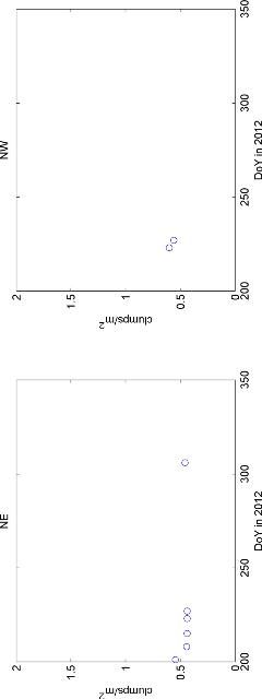
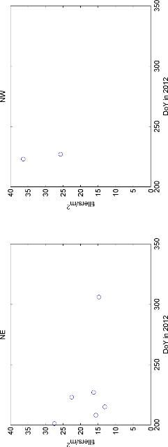
5.1 Clump and Tiller Count
The clumps and tillers were counted for each sampling length in each of the four sampling areas. Three representative clumps were chosen to determine the percentages of small, medium, and large tillers in the sampling area. Figure A-35 and A-36 show the clumps and tillers per square meter.
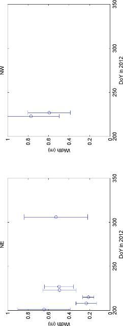
5.2 Clump Height and Width
Maximum clump height and width were measured by placing a tape measure at the soil surface adjacent to the stems to the maximum height of the clump. The clump width, parallel to the row, was measured at the base of the clump. Figures A-37 and A-38 show the average of the maximum clump heights and widths during MicroWEX-11.
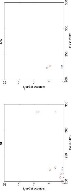
5.3 Wet and Dry Biomass
Using the sampling area, 10 tillers each of representative small, medium, and large were chosen from the three clumps in section 5.1. Each tiller was cut at the base, separated into leaves and stems, and weighed immediately. The samples were dried in the oven at 60ºC for one week for leaves and two weeks for stems. Figure A-39 shows the wet and dry biomass (in kg/m2) observed during MicroWEX-11 in the sampling area.
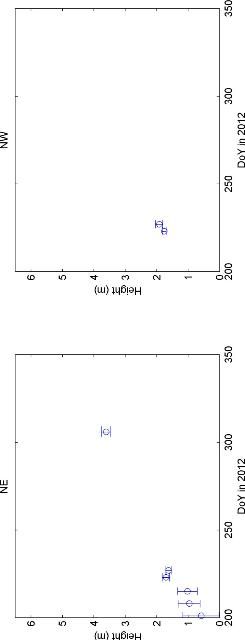
6. Vegetation Sampling at the Sweet Cornsite
Vegetation properties in two sampling locations as shown in Figure 3(c) were measured weekly during the field experiment. A vegetation sampling consisted of measurements of height, width, biomass, LAI, geometric description of the plant, and vertical distribution of moisture in the canopy. The crop density derived from the stand density (5.1 plants per m2) and row spacing (36?) was measured at the first sampling (DoY 250). Nine vegetation samplings were conducted on DoY 250, DoY 257, DoY 264, DoY 271, DoY 278, DoY 285, DoY 292, DoY 299, and DoY 306.
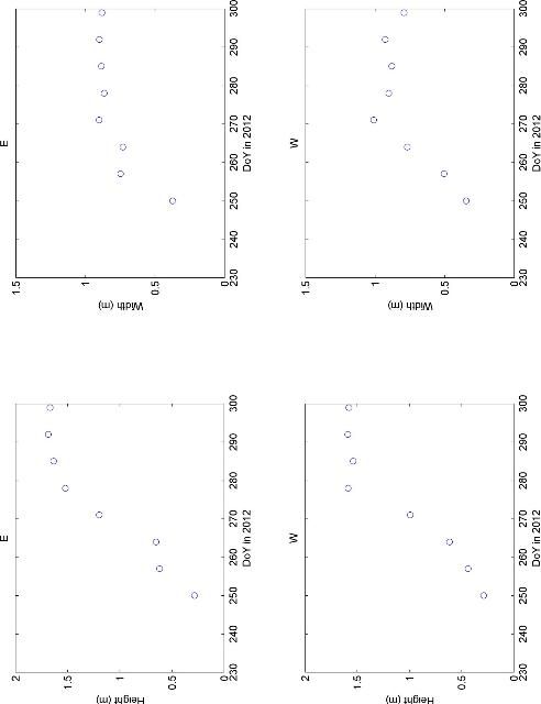
6.1 Height and Width
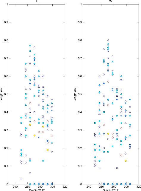
Crop height and width were measured by placing a measuring stick at the soil surface adjacent to the stem up to the maximum height of the crop. The maximum canopy width of the plant (parallel or perpendicular to the row) was also measured. Four representative plants were selected to obtain heights and widths inside each vegetation sampling area. Figure A-40 shows the average maximum crop heights and widths during MicroWEX-11.
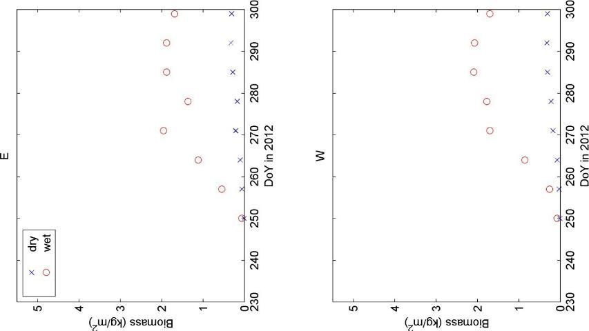
6.2 Wet and Dry Biomass
Each sampling included one row of corn in the four sampling locations. The sampling length started between two plants and ended at the next midpoint between plants that was greater than or equal to one meter away from the starting point. The plants within this length were cut at the base, separated into leaves, stems, and ears, and weighed immediately. The samples were dried in the oven at 60ºC for one week and weighed. Figure A-41 shows the wet and dry biomass observed during MicroWEX-11 for the four sampling areas.
6.3 LAI
Destructive LAI was measured by taking two representative plants in the sampling area and separating the leaves. The leaves and the rest of the plant were dried in an oven at 60°C for one week to measure the dry weight of the leaf and the dry biomass of the sample. The ratio of the leaf dry weight to the dry biomass was used to calculate the fraction of leaf (FLEAF) in Equation 1 (Boote 1994). The length and width of each individual leaf of the four sample plants were also measured. Assuming a leaf as an ellipse, the area of the leaves was summed and divided by the dry mass of the leaves to calculate the specific leaf area (SLA). The total dry biomass (DM) was found using the procedure in 5.2. Equation 1 was used to determine the destructive LAI.
Equation 1. ?????? = ???? · ?????????? · ??????
The LAI obtained is shown in Figure A-42.
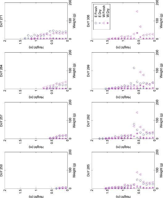
6.4 Vertical Distribution of Moisture in the Canopy
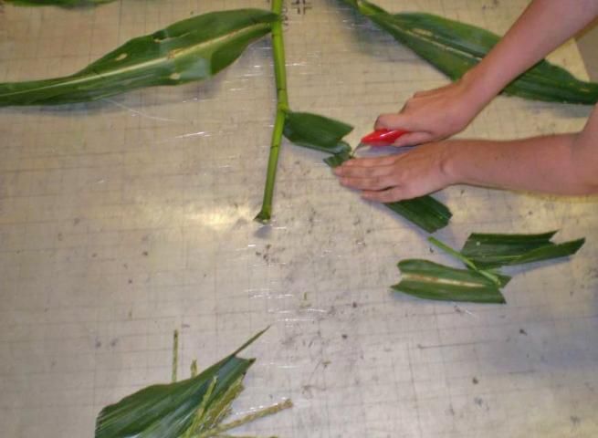
The wet and dry biomass of discrete vertical layers of individual corn plants was measured. Seven samplings were conducted during MicroWEX-11. Each sampling was conducted by selecting a representative plant at each sampling location. The plants were taken out of the ground with the roots still attached and taken indoors to prevent moisture loss. Each plant sample was carefully laid out on a metal sheet with grid spacing of 2 cm. The leaves were arranged to closely match their natural orientation in the field. The stem was cut every 10 cm as shown in Figure 15. The sample in each layer was weighed, both fresh and after drying in the oven at 60°C for 48 hours. Figure A-43 shows the wet and dry weights as a function of crop height during MicroWEX-11.
Credit: D. Preston, UF/IFAS
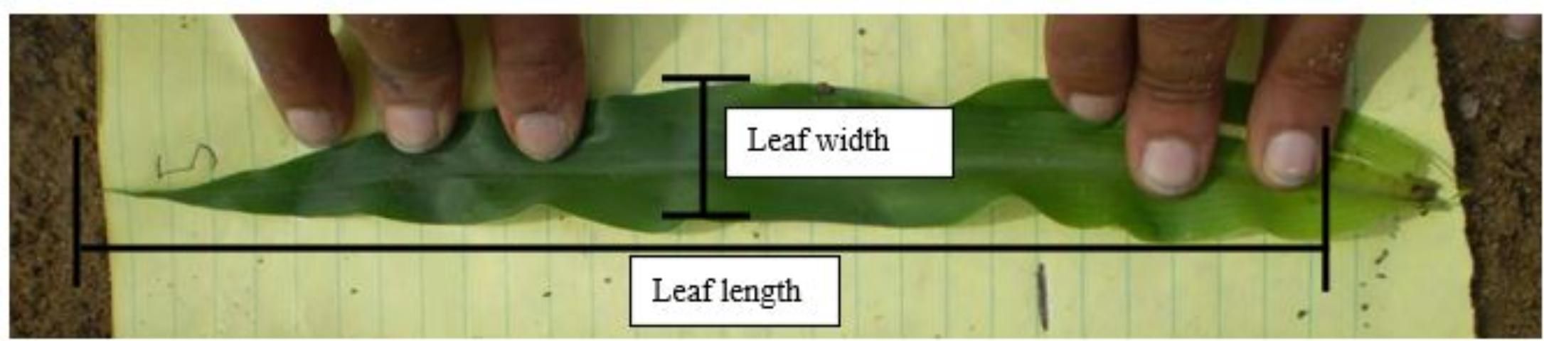
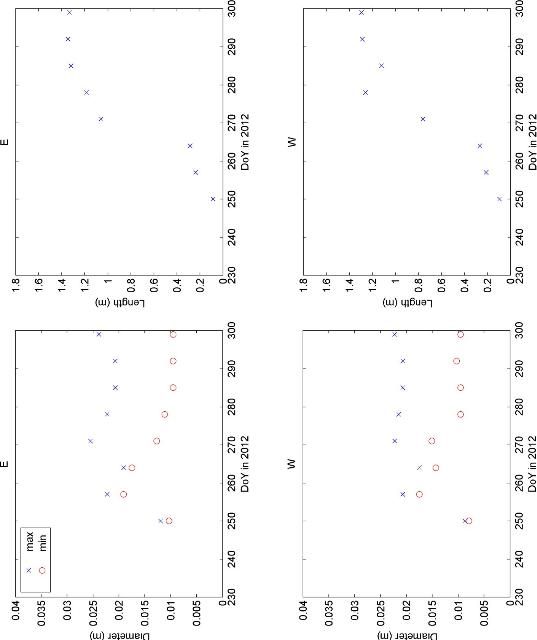
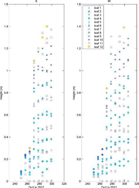
6.5 Geometric Description
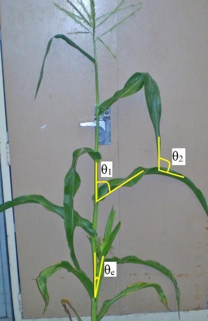
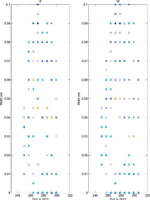
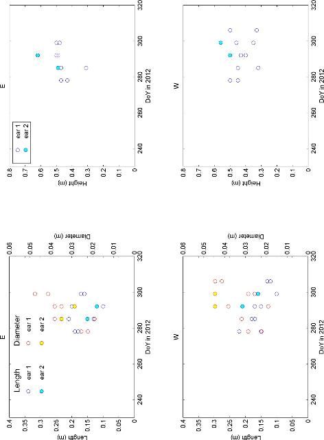
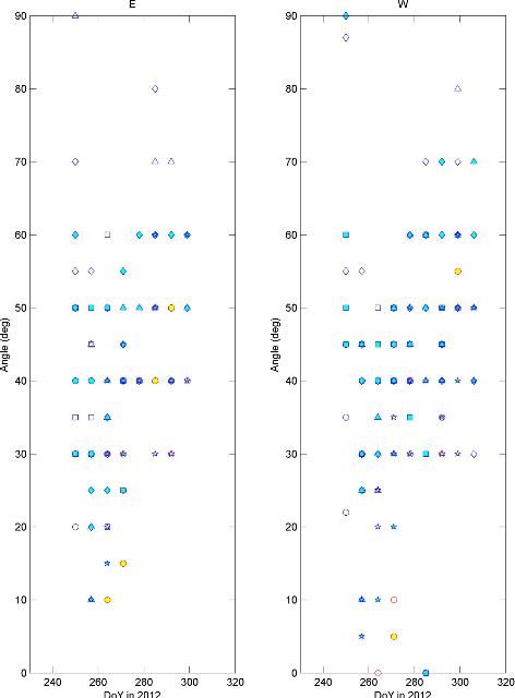
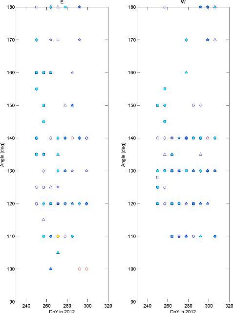
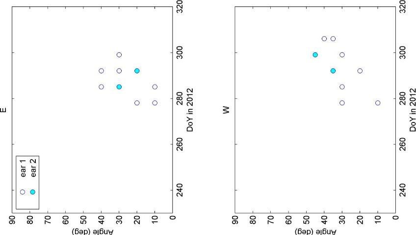
A geometric description of the plant consisted of the maximum length and width of each leaf of the sample plants, as shown in Figure 16. The stem circumference was measured by using a string to wrap around the base and around the tip of the plant to calculate the diameter of the stem. The ear length was measured while still in the husk from the base of the cob near the stem to the top, and the maximum circumference of the ear was measured by using a string. The stem length and diameter observed are shown in Figure A-44. Figure A-45 shows the height of each leaf. The leaf length and width are shown in Figures A-46 and A-47. The ear height, length, and diameter are shown in Figure A-48. The ear and leaf angles were measured from a digital photograph of a single plant taken while still in the field at each sampling area using a reference length such as a meter stick. The angle between the leaf and the stem (?1), the angle of the leaf fold (?2), and the ear angle (?e) were measured using an angle gage, as shown in Figure 17. See Figures A-49 and A-50 for the value of ?1 and ?2. Figure A-51 shows the ear angle for each ear.
Credit: D. Preston, UF/IFAS
Credit: R. Terwilleger, UF/IFAS
7. Well Sampling
7.1 Water Level Measurement
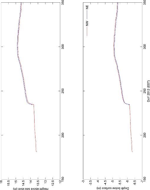
The water level measurement was processed by the Levelogger from Solinst Canada Ltd. The Leveloggers were installed at the northern wells in the elephant grass field and set to automatically record the water level every 30 minutes. The data were downloaded onto a laptop during the well sampling. Figure A-52 shows the water table elevation and depth during MicroWEX-11.
8. Soil Sampling
8.1 Soil Analysis
Soil sampling from three locations in the corn field was done on DoY 355. Samples included organic matter and texture analysis from depths of 0–10, 10, 20, 40, and 60 cm for the bare soil/corn site (Table 9), which were conducted by the UF/IFAS Extension Soil Testing Laboratory and the Soil and Water Science Soil Moisture Core Laboratory.
The soil physical properties for the corn field site (percentages are given on a weight basis).
8.2 Soil Surface Roughness
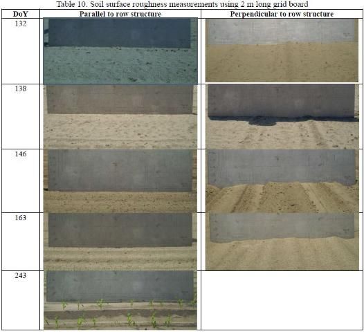
Soil roughness was measured in the bare soil field during the smooth period on DoY 132 and 138 and during the rough period on DoY 146 and 163 with a traditional grid board method (Table 10). Roughness measurements in the corn field were measured on DoY 243. The 2D surface profiles in directions parallel and perpendicular to the row structure during the bare soil period and parallel to the row structure during the corn field were measured using a 2 m long grid board. Jang et al. (2005) describes the grid board method in detail. Table 11 lists the root mean square height and correlation length measurements parallel and perpendicular to the row structure.
Soil surface roughness measurements of root mean square height (s) and correlation length (cl).
9. Observations
For the microwave radiometric observations at C-band, the horizontally polarized brightness temperatures were found to be more sensitive to soil moisture than vertically polarized brightness temperatures during the short vegetation cover periods (Figure A-1–A-3). As the vegetation grew, it effectively masked the contribution of microwave emission from soil resulting in sensitivity decrease at both polarizations. Due to its higher penetration capability, the observations at lower frequencies (longer wavelengths), such as the L-band, were more sensitive to soil moisture during the growing season than at the higher frequencies of C-band (Figure A-1–A-3). The σ0VV was more sensitive to the vertical structure of growing vegetation in the mid- and late-stages of crop growth (Figure A-4–A-6). The resonant frequency at leaf 8 shows a clear diurnal difference, as the afternoon resonant frequencies are higher than the morning values. This indicated that the leaf is losing water during the day and recovers at night (Figure A-7).
The average down-welling shortwave radiation average was 190.57 W/m2 during the elephant grass growing season while the average up-welling shortwave radiation was 40.18 W/m2 (Figure A-8). The average relative humidity was 78.97%, while the average air temperature was 295.03 K (Figure A-9). At the end of the elephant grass season when the temperature becomes cooler, the temperature near the soil remains high while the canopy temperature decreases (Figure A-10). The average thermal infrared temperature was 298.30 K, 294.73 K, and 298.35 K for the bare soil, elephant grass, and corn field (Figure A-11–A-13). There were dryer conditions during the bare soil period than the elephant grass and corn season (Figure A-32–A-34). The water table decreased after DoY 300 (Figure A-52).
During the beginning of the season when vegetation was low, diurnal variations in soil temperature were maximum while later in the season the diurnal variations were minimal. Diurnal variations for soil temperatures at 64 cm and below were minimal throughout the season (Figure A-14–A-22). The change in soil moisture in the deeper layers was minimal during light rains (Figure A-23–A-31).
The average clump density for the elephant grass was 0.5 clump/m2 (Figure A-35). The tiller density was higher in the NW vegetation sampling area (Figure A-36). The maximum height of the canopy was 3.6 m (Figure A-37). The average clump was 0.50 m wide (Figure A-38). The biomass of the plant on the final sampling was 2.8 kg/m2 (Figure A-39).
The maximum height of the sweet corn was 1.7 m for the east vegetation sampling area, while the west was slightly shorter at 1.6 m (Figure A-40). The maximum width of the sweet corn plant was 1.01 m at the west vegetation sampling area (Figure A-40). The biomass of the plant continued to increase until reaching an equilibrium after DoY 271 (Figure A-41). The LAI increased before reaching a maximum of 2 m2/m2, and then decreasing slightly due to leaf senescence (Figure A-42). During ear formation the moisture per 10 cm section in the plant was higher at the ear location (Figure A-43). The length of the stem increased until DoY 292 when it leveled out (Figure A-44). The average stem diameter at the top of the stem was 0.012 m while the average diameter at the base of the stem was 0.020 m (Figure A-44). The maximum number of main leaves was 12 leaves (Figure A-45). The maximum leaf length was 0.8 m (Figure A-46) and the maximum leaf width was 0.10 m (Figure A-47). Each plant had 1–2 ears, with the highest ear not exceeding 0.70 m above the base (Figure A-48). The ear located highest on the plant was bigger in both length and diameter than the other ears on the plant (Figure A-48). For the leaf angles, ?1 ranged from 0°–90° from the vertical (Figure A-49) while ?2 ranged from 90°–180° (Figure A-50). The ear angle, ?e, was larger for the bigger ears (FigureA-51).
10. Bare Soil Feed Log
11. Elephant Grass Field Log
12. Sweet Corn Field Log
13. References
Apogee Instruments, Inc. 2007. Infrared Radiometer Owner's Manual, Model: IRR-PN. Logan, UT: Apogee Instruments.
Boote, K. J. 1994. "Data Requirements for Model Evaluation and Techniques for Sampling Crop Growth and Development." In DSSAT Version 3.5, Volume 4, edited by Gerrit Hoogenboom, Paul W. Wilken, and Gordon Y. Tsuji. 215–220. Honolulu: University of Hawaii.
Campbell Scientific. 2006a. CNR1 Net Radiometer Instruction Manual. Logan, UT: Campbell Scientific.
Campbell Scientific. 2006b. Campbell Scientific Model HMP45C Temperature and Relative Humidity Probe Instruction Manual. Logan, UT: Campbell Scientific.
De Roo, R. D. 2002. University of Florida C-band Radiometer Summary. Ann Arbor: Space Physics Research Laboratory, University of Michigan.
De Roo, R. D. 2003. TMRS-3 Radiometer Tuning Procedures. Ann Arbor: Space Physics Research Laboratory, University of Michigan. De Roo, R. D. 2010. Personal communication.
Jang, M. Y., K. C. Tien, J. J. Casanova, and J. Judge. 2005. Measurements of soil surface roughness during the fourth microwave water and energy balance experiment: April 18 through June 13, 2005. Circular 1483. Gainesville: University of Florida Institute of Food and Agricultural Sciences. .
Nagarajan, K., P. W. Liu, R. DeRoo, J. Judge, R. Akbar, P. Rush, S. Feagle, D. Preston, and R. Terwilleger. "Automated L-Band Radar System for Sensing Soil Moisture at High Temporal Resolution." IEEE Geosci. and Remote Sens. Letters 11(2).
Van Emmerik, Tim H. M. 2013. "Diurnal differences in vegetation dielectric constant as a measure of water stress." PhD diss., Delft University of Technology.
14. Acknowledgments
The authors would like to acknowledge Mr. James Boyer and his team at the PSREU, Citra, Florida, for excellent field management. MicroWEX-11 was supported by grants from NASA-THP (Grant number: NNX09AK29G) and Netherlands Organization for Scientific Research (NWO) Veni Grant Program (ALW 863.09.015).
A. Field Observation
Missing Figure (FIGURE 61)
B. Julian Day Calendar
