Hydraulic Considerations for Citrus Microirrigation Systems
Introduction
Hydraulics is the study of the behavior of liquids as they move through channels or pipes. Hydraulic principles govern the flow of water through irrigation pipes. A basic understanding of these principles is necessary for understanding the design and operation of irrigation systems. This publication provides an introduction to hydraulics as it relates to citrus microirrigation.
Important Basic Terminologies
Head
Head is the energy in water (or other liquid) expressed in terms of the equivalent height of a water column above a given reference. Head at any point in the irrigation line is the sum of three components: static head, velocity head, and friction head.
Static or Elevation Head (He)
It is the vertical distance (e.g., ft) between the water inlet and the discharge point. It represents potential energy per unit mass of the water.
Velocity Head (Hv)
It is the energy (expressed in terms of head, ft) needed to keep irrigation water moving at a given velocity. It represents the kinetic energy per unit mass of water.
Friction Head (Hf)
Friction head (or loss) (Hf) is the energy needed to overcome friction in the irrigation pipes and is expressed in units of length (e.g., ft).
Pressure
It is the force per unit area. It is expressed in pounds per square inch (psi), Pascals, or Newtons per square meter.
Hydraulic Principles
A few basic hydraulic concepts related to water movement through pipes are particularly important to the design and proper operation of microirrigation systems.
1 ft3 of water = 62.4 pounds (lb)
1 gallon of water = 8.34 lb
Water weighs about 62.4 pounds per cubic foot (lb/ft3). This weight exerts a force on its surroundings, which is expressed as force per unit area or pressure (psi). The pressure on the bottom of a cubical container (1 x 1 x 1 ft) filled with water is 62.4 lb/ft2. Conversion to psi can be achieved as follows:
Pressure on 1 ft2 = 62.4 lb
1 ft 2 = (12)2 in2 = 144 in2
Pressure in psi for 1 foot of water = 62.4 lb/1 ft2 = 62.4 lb/144 in2 = 0.433 psi. Therefore to convert feet of water to psi and vice versa we can use:
Head (He) (ft) = Pressure (psi)/0.433 = 2.31 x pressure (psi) Eq. 1
The column of water does not have to be vertical. To calculate the static pressure between two points resulting from an elevation difference, only the vertical elevation distance between the two points needs to be known. However, other factors such as friction affect water pressure when water flows through a pipe.
Example 1
If the pressure gauge at the bottom of a tank filled with water displays 10 psi, determine the height of water (Ht) in the tank.
Ht = Pressure x 2.31 = 10 (psi) x 2.31 (ft/psi) = 23.1 ft
Velocity
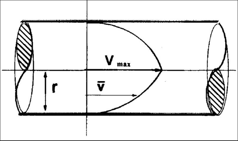
Velocity (V) is the average speed at which water moves through a pipe. Velocity is usually expressed in units of feet per second (ft/sec or fps). Water velocity in a pipe is greatest (Vmax) in the middle of the pipe and smallest near the pipe walls (Figure 1). Normally only the average velocity of water in the pipe is needed for hydraulic calculations. To avoid excessive pressure losses due to friction and excessive potentially damaging surge pressures, a rule of thumb for pipe sizing for irrigation pipelines is to limit water velocities to 5 ft/sec or less.
Flow
The relationship between flow rate and velocity is given by the equation of continuity, a fundamental physical law. This equation can be used to calculate flow by multiplying the velocity with the cross-sectional area of flow.
Q = A x V Eq. 2
or
V= Q/A Eq. 3
where,
Q = flow rate in ft3/sec,
A = cross-sectional area of flow in pipes in ft2 (A = 3.14 x D2/4),
V = velocity in ft/sec, and
D = pipe diameter (ft).
If pipe diameters change in sections of the pipe without any change in flow rate, the relationship between flow and velocity can be calculated by:
A1 x V1 = A2 x V2 Eq. 4
where,
A1 = cross-sectional area of flow for first section (ft2)
V1 = velocity in first section (ft/sec)
A2 = cross-sectional area of flow for second section (ft2)
V2 = velocity in second section (ft/sec)
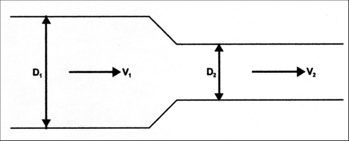
If the velocity is the same in a 2- and a 4-inch diameter pipe (Figure 2), the flow rate with the 4-inch pipe would be four times as large as the flow rate from the 2-inch diameter pipe. Note that the cross-sectional area is proportional to the diameter squared: (2 in.)2 = 4 in.2, while (4 in.)2 = 16 in2. Therefore, doubling the pipe diameter increases the carrying capacity of a pipe by a factor of 4.
Example 2
Determine the flow rate (gpm) in a 4-in Class 160 PVC pipe if the average velocity is 5 ft/s.
The I.D. for 4-in. pipe is 4.154 in. (See Table 1)
D = 4.154 in /12 = 0.346 ft
A = 3.14 x (0.346)2/4 = 0.094 ft2
Q = A x V = 0.094 ft 2 x 5 ft/s = 0.47 ft3/s (cfs)
Q = 0.47 cfs x 448 gal/cfs = 211 gpm
What would be the velocity if there was a transition to 3-in. Class 160 PVC with the same flow rate?
From Table 1, D2 = 3.230 in
D2 = 3.230 in /12 = 0.269 ft
A2 = 3.14 x 0.2692/4 = 0.057 ft2
Rearranging Eq. 4 results in:
V2 = (A1 x V1) / A2
= (0.094 ft2 x 5 ft/sec)/0.057 ft2= 8.25 ft/sec
Pressure and Flow
As water moves through any pipe, pressure is lost due to turbulence created by the moving water. The amount of pressure lost in a horizontal pipe is related to the velocity of the water, pipe diameter and roughness, and the length of pipe through which the water flows. When velocity increases, the pressure loss increases. For example, in a 1-in. schedule 40 PVC pipe with an 8 gpm flow rate, the velocity will be 2.97 fps with a pressure loss of 1.59 psi per 100 ft. When the flow rate is increased to 18 gpm, the velocity will be 6.67 fps, and the pressure loss will increase to 7.12 psi per 100 ft of pipe.
Bernoulli's Theorem
At any point within a piping system, water has energy associated with it. The energy can be in various forms including pressure, elevation, velocity, or friction (heat). The energy conservation principle states that energy can neither be created nor destroyed. Therefore, the total energy of the fluid at one point in the system must equal the total energy at any other point in the system, plus any energy that might be transferred into or out of the system. This principle is known as Bernoulli's Theorem and can be expressed as (Eq. 5):
Total head = He + Hp + Hv Eq. 5
He1 + Hp1 + Hv1 = He2+ Hp2+ Hv2
+ Hf Eq. 6
where,
He = Static head or elevation head in feet above some reference point (ft)
Hp = P/G (P = Pressure (psi) and G = specific weight (lb/ft3) of water) (ft)
Hv = Velocity head (ft) = V2/2g,
V = velocity in ft/s,
g = gravitational constant 32.2 ft/s2,
Hf = friction head (ft), and subscripts 1 and 2 refer to two points in the fluid system.
The friction head (Hf) can be calculated by the Hazen-Williams equation discussed in the next section. Velocity head is usually a small fraction of the total hydraulic head in a pressurized irrigation system, therefore, for the purpose of design it can be ignored (e.g., for v = 5ft/s, Hv= 0.39 ft).
Example 3
The pressure at the pump of an irrigation system is 30 psi. A microsprinkler is located at another location, which is 10 ft higher than the pump. What is the static water pressure at the microsprinkler (assume no flow and thus no friction loss)? For convenience, the pump can be used as the elevation datum.
The total energy at the pump is determined:
H = Pc + E Eq. 7
where,
H = energy head (ft)
P = pressure head (psi)
E = elevation (ft)
c = conversion constant to convert psi to ft (2.31 ft/psi).
In this example, since there is no water flowing, the energy at all points of the system is the same. Pressure at the microsprinkler is found by solving equation for P:
Reorganization of Eq. 7 results in P = (H - E)/c
P = (30*2.31 ft -10 ft) / 2.31 (ft/psi) = 25.7 psi = 25.7*2.31 ft = 59.37 ft
Hazen-Williams Equation
Water flowing in a pipe loses energy because of friction between the water and pipe walls and turbulence. In the above example, when the microsprinkler is operating, pressure will be less than the 25.7 psi due to friction loss in the pipe and the micro tubing. It is important to determine the amount of energy (or friction head) lost in pipes in order to properly size them. The Hazen-Williams equation is extensively used for designing water-distribution systems. The friction-loss calculations for most pipe sizes and water temperatures encountered under irrigation system conditions are shown in Table 1 and Table 2. The values in Table 1 and Table 2 are computed using the Hazen-Williams equation. A more accurate equation, Darcy-Weisbach, is sometimes used for smaller pipes or when heated water is being piped; however, the computations are more difficult. The Hazen-Williams equation can be expressed as:
Hf = (4.73 x (Q/C)1.85 L)/D4.87 Eq. 8
where,
Hf = friction loss (feet)
Q = flow rate (cubic feet per second (cfs))
D = inside pipe diameter (in)
L = length of pipe (feet), and
C = friction coefficient or pipe roughness
For most irrigation systems a value of C=150 (for plastic pipes) is used which reduces the above Equation to:
Hf = (0.000446 x Q1.85 x L)/D4.87 Eq. 9
The above Equation can also be expressed as:
Hf = (0.000977 x Q1.85 x L)/D4.87 Eq. 10
where all the terms and units are as defined except that Q has a unit of gallons per minute (gpm).
Friction loss in pipes depends on: flow (Q), pipe diameter (D), and pipe roughness (C). The smoother the pipe, the higher the C value. Increasing flow rate or choosing a rougher pipe will increase energy losses, resulting in decreased pressures downstream. In contrast, increasing inside diameter decreases friction losses and provides greater downstream pressure.
Example 4
Determine the pipe friction loss in 1,000 ft of 8-inch Class 160 PVC pipe, if the flow rate is 800 gpm.
From Table 1, the I.D. of 8-inch pipe is 7.961 inches. From Equation 10:
Hf = (0.000977 x (800)1.85 x 1000)/7.9614.87 )
Hf = 9.39 ft
Because of friction, pressure is lost whenever water passes through fittings, such as tees, elbows, constrictions, or valves. The magnitude of the loss depends both on the type of fitting and on the water velocity (determined by the flow rate and fitting size). Pressure losses in major fittings such as large valves, filters, and flow meters, can be obtained from the manufacturers. To account for minor pressure losses in fittings, such as tees and elbows, Table 3 can be used. Minor losses are sometimes aggregated into a friction loss safety factor (10% is frequently used) over and above the friction losses in pipelines, filters, valves, and other elements. Although the Hazen- Williams equation facilitates easy manual computations for pipe friction (provided a correct value of C is used), more complex and accurate methods (e.g., Reynolds number based Equations) are also available. These complex equations are used in several of the currently available computer programs that are used to design microirrigation systems.
Hydraulics of Multiple Outlet System
For a pipeline with multiple outlets at regular spacing along mains and submains, the flow rate downstream from each of the outlets will be effectively reduced. Since the flow rate affects the amount of pressure loss, the pressure loss in such a system would only be a fraction of the loss that would occur in a pipe without outlets. The Christiansen lateral line friction formula is a modified version of the Hazen-Williams Equation and was developed for lateral lines with sprinklers or emitters that are evenly spaced with assumed equal discharge and a single pipe diameter. The Christiansen formula introduces a term known as multiple outlet factor "F" in the Hazen-Williams equation to account for multiple outlets:
Hfl = F x Hf (Hf from Equation 8) Eq. 11
For flow in gpm and diameter in inches the expanded form of the above Equation becomes:
Hfl = F x (L/100) x [ { k x (Q/C)1.85}/D 4.871
where,
Hfl = head loss due to friction in lateral with evenly spaced emitters (ft)
L = length of lateral (ft)
F = multiple outlet coefficient (see Table 4)
= [1/(m + 1)] + [1/2n] + [(m + 1)0.5/(6n2)]
m = velocity exponent (assume 1.85),
n = number of outlets on lateral,
Q = flow rate in gpm,
D = inside pipe diameter in inches,
k = a constant 1,045 for Q in gpm and D in inches, and
C = friction coefficient: 150 for PVC or PE pipe (use 130 for pipes less than 2 inches)
Example 5
Determine the friction loss in a 0.75-inch poly lateral that is 300 ft long with 25 evenly spaced emitters on each side of the riser. Each emitter has a discharge rate of 15 gallons per hour (gph).
Flow rate into each half of the lateral is: 25 emitters x 15 gph each = 375 gph or 375 gph / 60 min = 6.3 gpm
From Table 2, the I.D. of 0.75-inch poly is 0.824 inches
From Table 4, F = 0.355 (average of 0.36 and 0.35)
C = 130 for 0.75-inch poly tubing
Hfl= 0.355 (300/100)(1045 x (6.3/130)1.85)/0.8244.87
= 10.57 ft = 10.57 ft / 2.31 psi/ft = 4.57 psi
Hydraulic Characteristics of Lateral Lines
The goal of a good irrigation system is to have high uniformity and ensure (as much as feasible) that each portion of the field receives the same amount of water (as well as nutrients and chemicals). As water flows through the lateral tubing, there is friction between the wall of the tubing and the water particles. This results in a gradual (but not uniform) reduction in the pressure within the lateral line. The magnitude of pressure loss in a lateral line depends on flow rate, pipe diameter, roughness coefficient (C), changes in elevation, and the lateral length.
When a lateral line is placed up-slope, emitter flow rate decreases most rapidly. This is due to the combined influence of elevation and friction losses. Where topography allows, running the lateral line down-slope can produce the most uniform flow since friction loss (negative) and elevation factors (positive) cancel each other out to some degree.
Friction loss is greatest at the beginning of the lateral. Approximately 50% of the pressure reduction occurs in the first 25% of the lateral's length. This occurs because as the flow rate decreases, friction losses decrease more rapidly. The lengths of laterals have a large impact on uniform application. For a given pipe diameter and emitter flow rate, too long laterals is one of the most commonly observed sources of non-uniformity in microirrigation systems. In general, longer lateral length results in less uniform application rate.
Water Hammer
Water hammer is a hydraulic phenomenon which is caused by a sudden change in the velocity of the water. This velocity change results in a large pressure fluctuation that is often accompanied by loud and explosive-like noise. This release of energy is due to a sudden change in momentum followed by an exchange between kinetic and pressure energy. The pressure change associated with water hammer occurs as wave, which is very rapidly transmitted through the entire hydraulic system. If left uncontrolled, water hammer can produce forces large enough to damage the irrigation pipes permanently.
When water is flowing with a constant velocity through a pipe and a downstream valve is closed, the water adjacent to the valve is stopped. The momentum in water creates a pressure head which results in compression of water and expansion of the pipe walls. These pressures can be several times the normal operating pressure and result in broken pipes and severe damage to the irrigation system. The high pressures resulting from the water hammer can not be effectively relieved by a pressure relief valve due to the high velocity of the pressure wave (pressure wave can travel at more than 1,000 ft per second in PVC pipe). The best prevention of water hammer is the installation of valves that can not be rapidly closed, and the selection of air vents with the appropriate orifice which do not release air too rapidly. Pipelines are usually designed to maintain velocities below 5 fps in order to avoid high surge pressures from occurring. Surge pressures may be calculated by the following (Eq. 12):
P = {0.028 (Q x L) } /D2 x T Eq. 12
where,
Q = flow rate (gpm)
D = pipe I.D. (inches)
P = surge pressure (psi)
L = length of pipeline (feet)
T = time to close valve (seconds)
Example 6
For an 8-inch Class 160 PVC pipeline that is 1,500 feet long and has a flow rate of 750 gpm, compare the potential surge pressure caused when a butterfly valve is closed in 10 seconds to a gate valve that requires 30 seconds to close.
From Table 1, diameter of 8 inch pipe is 7.961 inches
Butterfly valve (Pbv):
Surge Pressure (Pbv) = 0.028 x (750 x 1500) / (7.9612 x 10) = 49.7 psi
Gate valve (Pgv):
Surge Pressure (Pgv) = 0.028 x (750 x 1500) / (7.9612 x 30) = 16.57 psi
From the above example, it is clear that increasing the closing time for valves can reduce the surge pressure.
Head Losses in Lateral Lines
Microsprinkler field installations typically have 10-20 gph emitters. Emitters are normally attached to stake assemblies that raise the emitter 8-10 inches above the ground, and the stake assemblies usually have 2-3 ft lengths of 4-mm spaghetti tubing. The spaghetti tubing is connected to the polyethylene lateral tubing with a barbed or threaded connector. The amount of head loss in the barbed connector can be significant, depending on the flow rate of the emitter and the inside diameter of the connector. The pressure loss in a 0.175 inch barb x barb connector is shown in Figure 3. At 15 gph, about 1 psi is lost in the barbed connection alone.
Missing Figure (FIGURE 8)
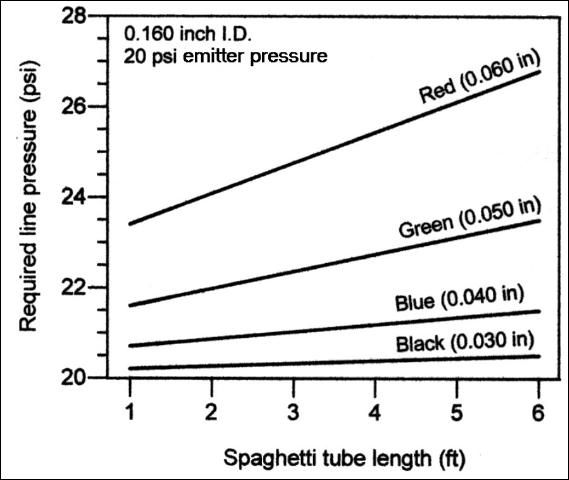
In addition to the lateral tubing connection, there will be pressure losses in the spaghetti tubing. Figure 4 shows the pressure required in the lateral line to maintain 20 psi at the emitter for various emitter orifices and spaghetti tubing lengths. Note that with the red base emitters (0.060 in. orifice), an additional 25-30% pressure is required in the lateral tubing to maintain 20 psi at the emitter.
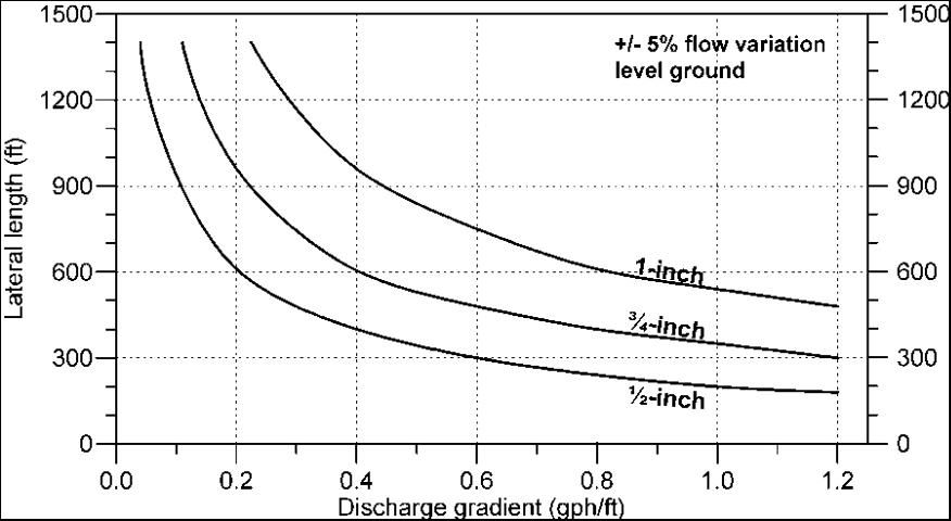
It is important to realize the hydraulic limits of irrigation lateral lines to efficiently deliver water. Oftentimes when resetting trees, 2 or more trees are planted for each tree taken out. If a microsprinkler is installed for each of the reset trees, the effects of increased emitters on the system uniformity and system performance can be tremendous. Not only will friction losses increase and average emitter discharge decrease, but system uniformity and efficiency will decrease. Figure 5 shows the maximum length of lateral tubing that is possible while maintaining ± 5% flow variation on level ground with a 20 psi average pressure. The discharge gradient is calculated by dividing the emitter flow rate (gph) by the emitter spacing (ft).
The maximum number of microsprinkler emitters and maximum lateral lengths for 0.75, and 1-inch lateral tubing is given in Table 5 and Table 6. Similar information for drippers with 0.5, 0.75, and 1-inch lateral tubing is given in Table 7, Table 8, and Table 9. All calculations are based on ±5% allowable flow variation on level ground. By knowing the emitter discharge rate, spacing, and tubing diameter, the maximum number of emitters and the maximum lateral length can be determined.
Example 7
Determine the maximum allowable run length for 0.75-inch lateral tubing with 10 gph emitters spaced at 12-ft intervals.
Discharge gradient = 10 gph / 12 ft = 0.83 gph/ft
From Figure 5, maximum run length corresponding to 0.83 gph/ft gradient is about 380 ft (32 trees).
Example 8
Determine the maximum allowable run length for 0.75-inch lateral tubing with 12 gph emitters spaced at 10-ft intervals.
For 12 gph and 10-ft spacing, (Table 5):
Maximum number of emitters: 31
Maximum lateral length: 313 ft
Alternatively, Figure 5 can be used to compute the maximum lateral length for +/-5% flow variations.
Discharge gradient = 12 gph/10 ft = 1.2 gph/ft
Corresponding value for 1.2 gph/ft from Figure 5 is 300 ft.
Example 9
Using Tables 7 to 9, determine the maximum allowable run length for 0.75-inch lateral tubing with 1.0 gph drip emitters spaced at 30-inch intervals.
From Table 8 for 1.0 gph at 30-inch spacing,
Maximum number of emitters: 227
Maximum lateral length: 568 ft
References
Boswell, M. J. 1990. Micro-irrigation design manual. James Hardie Irrigation, Inc. El Cajon, CA.
Burt, C. M. and S. W. Styles. 1999. Drip micro irrigation for trees, vines, and row crops. San Luis Obispo, CA: Irrigation Training and Research Center, California Polytechnic State University.
Clark, G. A., A. G. Smajstrla, and D. Z. Haman. 1994. Water hammer in irrigation systems. UF/IFAS Extension. Circ. 828.
Howell, T. A., D. S. Stevenson, K. A. Aljibury, H. M. Gitlin, A.W. Warrick, and P. A. C. Raats. 1980. Design and operation of trickle (drip) systems. Chapter 16. In: Jensen, M.E. (Ed.) Design and Operation of Farm Irrigation Systems. ASAE Monograph No. 3. American Society of Agricultural Engineers, St. Joseph, MI.
Hunter Irrigation. 1997. Irrigation hydraulics student manual. Hunter Industries, Inc. San Marcon, CA.
Tables
Maximum allowable flow rate and friction losses per 100 feet for Class 160 PVC IPS pipe. Flow rate is based on a maximum velocity of 5 fps (friction loss calculated at maximum flow rate by Hazen-Williams equation).
Maximum allowable flow rate and friction losses per 100 feet for Polyethylene (PE) SDR 15-80 psi pressure-rated tubing based on a maximum velocity of 5 fps (friction loss calculated at maximum flow rate by Hazen-Williams equation).
Maximum number of microsprinkler emitters and maximum lateral lengths for ¾-inch lateral tubing diameter (± 5% allowable flow variation on level ground: based on Bowsmith ¾-inch tubing, I.D.=0.818 in.).
Maximum number of microsprinkler emitters and maximum lateral lengths for 1-inch lateral tubing diameter (± 5% allowable flow variation on level ground: based on Bowsmith 1-inch tubing, I.D.=1.057 in.).
Maximum number of drip emitters and maximum lateral lengths for ½-inch lateral tubing diameter (± 5% allowable flow variation on level ground: based on Bowsmith P720P48 (½-inch) tubing, I.D.=0.625 in.).
Maximum number of drip emitters and maximum lateral lengths for ¾-inch lateral tubing diameter (±5% allowable flow variation on level ground: based on Bowsmith ¾-inch tubing, I.D.=0.818 in.).
