MENU

AskIFAS Powered by EDIS

Net Irrigation Requirements for Florida Turfgrass Lawns: Part 3—Theoretical Irrigation Requirements1

Consuelo C. Romero and Michael D. Dukes 2

Introduction

Turfgrasses are used in urban areas to provide multiple benefits to society and the environment. They cover millions of acres of home lawns, commercial properties, roadsides, parks, etc. But an important question is whether turfgrasses are properly managed. Many critics emphasize that turfgrasses demand too much urban water in a time when water resources are scarce. While indoor water use remains fairly constant throughout the year, outdoor water use increases during the spring and summer. Flattening the peak demand is an objective of water agencies (Beard and Kenna 2006); better irrigation management would result in less fertilizer and pesticide use, which would be better for the environment.

Urban landscape irrigation is one of the largest growing water use sectors in Florida. The state's Water Management Districts have been working collectively to find ways to assist urban water users to irrigate more efficiently and to enhance planning and regulatory programs in order to conserve water. There is adequate research information to make specific recommendations, such as the specific cultural practices or systems approaches that could be applied to decrease turfgrass water use. Those recommendations could be used immediately to conserve water and maintain turfgrass quality and its functional benefits to society.

The calculation of net irrigation requirements for turfgrass is essential for determining water allocation and can help to determine irrigation scheduling. This series of publications explains the process of estimating net irrigation requirements for Florida turfgrasses. The process used here gives a long-term (30-year) historical analysis of turfgrass monthly net irrigation requirements. The first article in the series explains how the weather data was gathered and checked for quality; the second article shows the calculation of evapotranspiration for selected sites throughout the state (plus one in Alabama, to cover the west side of the Florida Panhandle); and the third and final article outlines the results of the net irrigation estimation. Since Florida's urban landscape water demand is expected to grow considerably over the next few decades, the use of current information in terms of turfgrass irrigation needs will provide urban irrigators with information to help them reduce water volumes applied and conserve water.

Net irrigation is the depth of water needed to fulfill the evapotranspiration (ET) requirement in addition to the amount of precipitation available to a growing crop, for a disease-free crop growing in large fields under non-restricting water conditions and under adequate fertility (Allen et al. 2007). Turfgrass is mostly under irrigation and is considered the largest irrigated non-agricultural crop in the United States (Hoffman et al. 2007). Knowing when to irrigate and how much water to apply can help to minimize water and energy use (Evans et al. 1996). It has been found that water application in excess of that required can largely be attributed to human factors and not to plant needs (Beard and Green 1994).

In this study, a soil water balance is used to calculate irrigation requirements for Florida turfgrass lawns based on 30 years of historical weather data. The first publication in the series shows that the weather data has been quality checked (Net Irrigation Requirements for Turfgrass Lawns: Part 1—Report of Gathered Weather Data and Quality Check https://edis.ifas.ufl.edu/publication/ae480). In the second publication in the series, the reference evapotranspiration has been calculated and analyzed (Net Irrigation Requirements for Turfgrass Lawns: Part 2—Reference Evapotranspiration Calculation https://edis.ifas.ufl.edu/publication/ae481). The estimated irrigation requirements are presented on a monthly basis, and each monthly value represents the average of the 30-year period. These monthly values can be recommended when irrigation will most likely be needed during the year. These recommendations should be analyzed carefully since we are assuming that the irrigated landscape is covered only by turfgrasses. A more detailed analysis must be performed for mixed landscapes or areas where ornamental plants dominate.

Objective

The objective of this report is to estimate net irrigation, effective rainfall, and drainage by using a water balance equation for ten locations in Florida and one in Alabama from data during the 30-year period of 1980–2009.

Methodology

Irrigation Estimation Using a Water Balance Model

The soil water balance presented by Dukes (2007) was calculated on a daily basis for thirty years (1980-2009) for 10 sites in Florida and one in Alabama. Daily gain and loss of water was computed by the equation once the maximum allowed depletion (MAD) value was reached. The soil water balance equation, in units of inches, was as follows:

SWt = SWt-1 - ETct-1 + Rt-1 + It-1 - Dt-1 - Rofft-1 (Eq. 1)

where SWt is the soil water on day 't', SWt-1 is the soil water content on day 't-1', ETt-1 is the crop evapotranspiration, Rt-1 is rainfall (https://edis.ifas.ufl.edu/publication/ae480), It-1 is net irrigation, Dt-1 is drainage, and Rofft-1 is runoff. ETc was calculated as the product of ETo (https://edis.ifas.ufl.edu/publication/ae481) by a Kc (or crop coefficient) that varied monthly. ETc was subtracted from the soil water store on a daily basis until the root zone reached a MAD level. The MAD value established for warm-season turfgrass has been suggested as 0.5 (Allen et al. 1998). We simulated the effect of two root zones at 8 and 12 in. These are the most frequent root depths found for warm-season turfgrasses (Shedd et al. 2008; Huang et al. 1997; Peacock and Dudeck 1985; DiPaola et al. 1982). During the simulations, irrigation was triggered to refill the soil profile to field capacity when moisture conditions reached the MAD level. Rainfall beyond field capacity was assumed to be lost from the system due to drainage. The most dominant soils covering the urban areas were selected in order to simulate a "high" and a "low" soil water holding capacity as shown in Table 1. Runoff on these coarse soils was assumed to be negligible. Three sets of monthly turfgrass crop coefficients for North, Central, and South Florida were used for the simulations, and values are shown in Table 2 (Jia et al. 2009; Davis and Dukes 2010).

The mean net irrigation requirements included the effect of using different root zones and soil water holding capacity levels. The 5-in-10 and 2-in-10 (80th percentile) irrigation was also analyzed. The 5-in-10 irrigation requirements represent the median or 50th percentile and should be numerically similar to the mean irrigation requirement if the net irrigation values distribution is normal. The 2-in-10 net irrigation values represent amounts that fulfill the net irrigation requirement 80% of the time and would represent the amount of irrigation to maintain irrigation needs through a drought with a frequency of occurrence 2 years in every 10. The Southwest Florida Water Management District has permitted supplemental irrigation quantities in this manner (SWFWMD 2011).

Results and Discussion

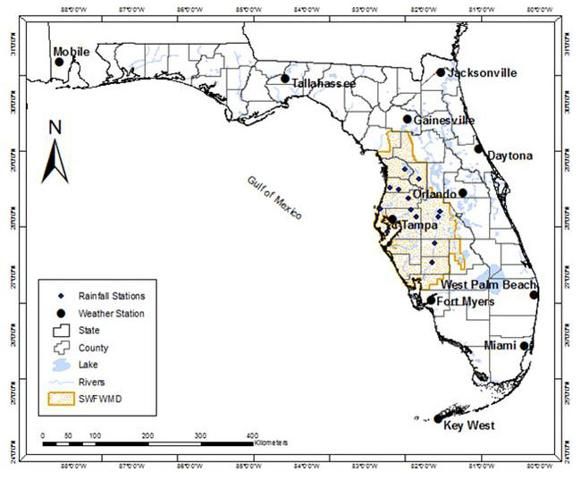
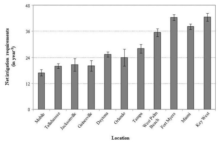
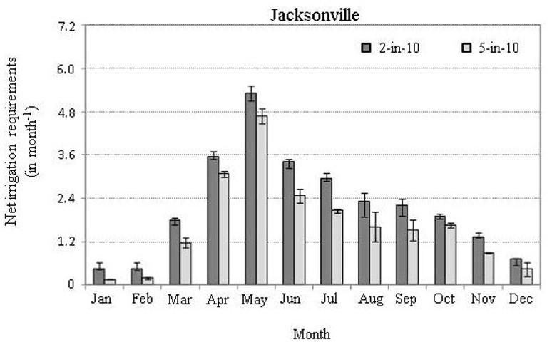
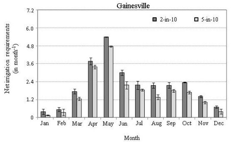
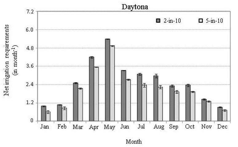
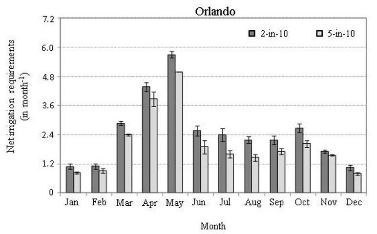
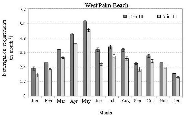
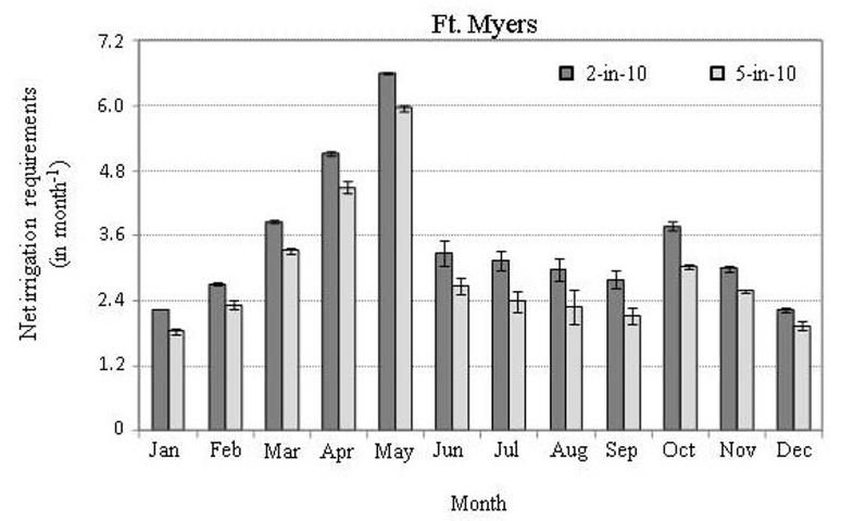
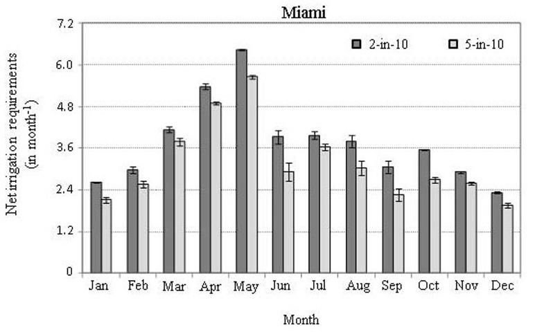
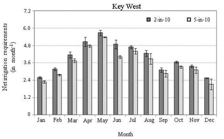
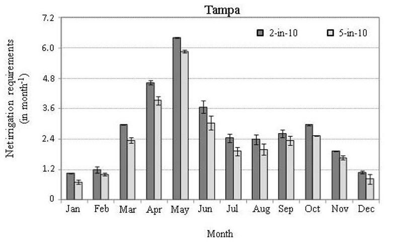
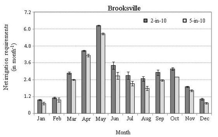
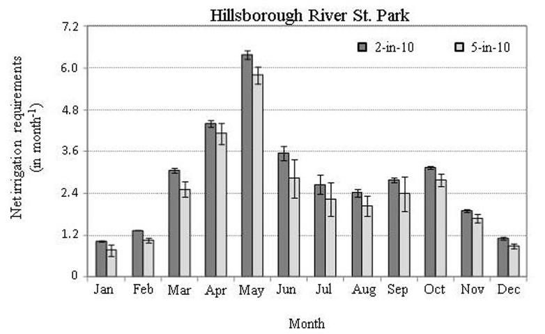
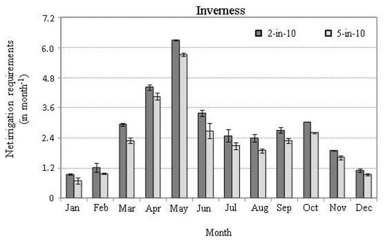
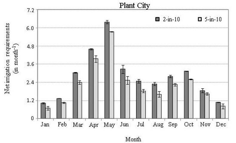
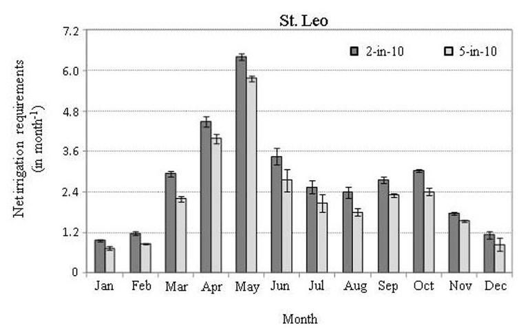
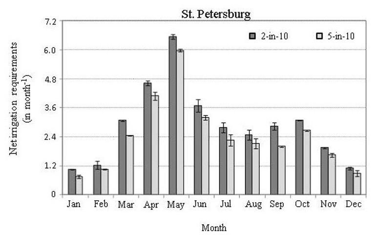
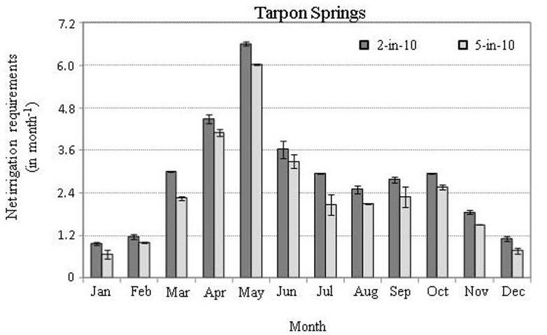
Thirty years (1980-2009) of daily net irrigation requirements were calculated for 10 sites in Florida and one in Alabama (Figure 1). The locations have been grouped into five zones based on geographical distribution: Florida Panhandle (Mobile and Tallahassee), North Florida (Jacksonville and Gainesville), Central Florida (Daytona and Orlando), Southwest Florida (Tampa, Brooksville, Hillsborough River State Park, Inverness, Plant City, St. Leo, St. Petersburg, and Tarpon Springs), and South Florida (West Palm Beach, Ft. Myers, Miami, and Key West). A comparison of the mean annual irrigation amounts per site is shown in Table 3 and Figure 2. The mean monthly net irrigation requirements, drainage, and effective rainfall on a monthly basis were calculated by using 8 and 12 in root zone and are shown in Table 4. The 5-in-10 (50th percentile) and the 2-in-10 (80th percentile) irrigation requirements are shown in Table 5 (average of 8 and 12 in root zone). These data are also shown as graphs in Figures 3 through 20.

The mean annual net irrigation ranged from 16.7 in y-1 in Mobile (Florida Panhandle) to 41.7 in y-1 in Fort Myers. For Key West (South Florida), the estimated net irrigation requirement was 38.5 in y-1 (Table 3). According to the second article in this series (https://edis.ifas.ufl.edu/publication/ae481), Mobile showed a higher mean yearly rainfall than Key West, with 69.7 in y-1 and 41.7 in y-1, respectively. Tampa and nearby sites (Southwest Florida) showed an annual mean net irrigation requirement of 27.6 in y-1. The yearly standard deviation values are also shown in Table 3, and the average standard deviation is 2.1 in y-1. This value reflects the variation of using different root zones and soil types, but also includes the variability of climate during the 30 years of evaluation. The difference between using 8 or 12 in root zone was 1.7 in y-1on average. Net irrigation requirements were higher when an 8 in root zone was simulated. At that depth, soil retains less water; rainfall is less effective in supplying the amount of water needed; and drainage is higher than in a deeper soil, making irrigation more frequently required.


Figure 1. Map showing weather station locations (large dots) and rain gauges (small dots).
Figure 1.  Map showing weather station locations (large dots) and rain gauges (small dots).


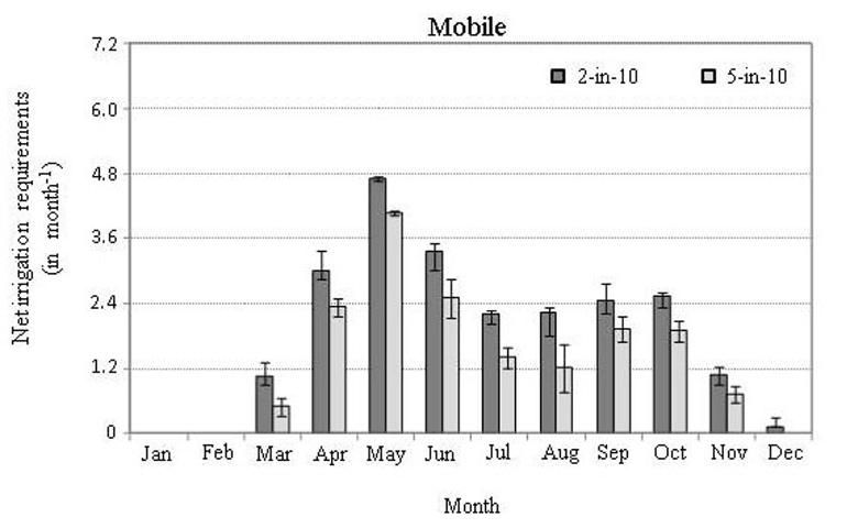
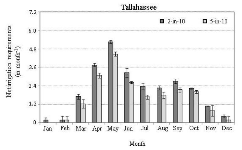
The average mean monthly distribution of net irrigation, drainage, and effective rainfall using 8 and 12 inch root zones is shown in Table 4. Irrigation requirements increased from December to May, decreased during the summer season, and then increased slightly again during September and October. The highest irrigation requirement in a year was calculated in May, with approximately 5.2 in month-1. Minimum irrigation was calculated for the winter months in higher latitudes (e.g., Mobile and Tallahassee) when no irrigation was required and corresponded to the grass dormant season, specifically in January. The opposite was calculated in southern latitudes where irrigation is required almost year-round (e.g., Fort Myers, Miami, and Key West). We found out that the irrigation requirements for South Florida were in agreement with measured ETc data found in the literature, in spite of our overestimated ETo for the area (https://edis.ifas.ufl.edu/publication/ae481). For example, ETo was calculated as 65.3 in y-1, and the estimated irrigation as 37.6 in y-1 in Miami. Stewart and Mills (1967) measured turf evapotranspiration in South Florida, finding a water demand of 42.8 in y-1. The overestimated ETo data did not impact the net irrigation estimate.

Monthly distribution of the estimated irrigation was very similar among the locations identified in Southwest Florida. The calculated drainage and effective rainfall values were higher during June to September in all cases.

During a drought year, additional irrigation is required to meet plant water requirements. Accordingly, the Southwest Florida Water Management District (SWFWMD) consumptive use permits allow for the 2-in-10 net irrigation requirement instead of the average or the median (5-in-10) irrigation requirement. The 2-in-10 and 5-in-10 monthly net irrigation requirements are shown in Table 5, and each value represents the average of using 8 and 12 inch root zones. The mean maximum 2-in-10 net irrigation requirement was approximately 5.9 in month-1, which represents 14% more than the mean net irrigation requirement. The mean monthly net irrigation values shown in Table 4 differed slightly from the median values (5-in-10 irrigation requirements shown in Table 5). The median gives the middle value of an ordered set of values, in this case the estimated net irrigation. Figures 3 through 20 show several graphs of the 2-in-10 and 5-in-10 irrigation requirements at each location. Error bars represent the standard deviation due to root zone differences. It is important to note that the gross irrigation requirement would result in more water allocated to account for reasonable irrigation inefficiencies.


Figure 2. Yearly average net irrigation requirement in all locations in Florida. Error bars represent the standard deviation due to different root zones and soil types across years.
Figure 2.  Yearly average net irrigation requirement in all locations in Florida. Error bars represent the standard deviation due to different root zones and soil types across years.


Summary

The irrigation requirements for turfgrass lawns in 10 cities in Florida and one in Alabama were estimated and analyzed for a 30-year period (1980-2009). The annual estimated irrigation requirements ranged from 16.7 in to 41.7 in y-1 in Mobile and Fort Myers, respectively. The results showed that the estimated irrigation was less in the Florida Panhandle but gradually increased its demand in Central and South Florida. On average, monthly irrigation requirements increase two times a year, from April to June (high peaks in May with 5.2 in month-1, approximately), and from October to November (maximum in October with 2.4 in month-1, approximately). These peaks of estimated irrigation demands are related to rainfall trends that showed less rain is observed from October to May, compared to the rainy season occurring from June to September. Evapotranspiration increases in the first months of the year, with the highest peak calculated for May, and then it decreases gradually in the following months. The estimated irrigation requirements for locations in Southwest Florida showed similar trends because reference evapotranspiration was calculated from data of one weather station. However, minor changes in the estimated irrigation were due to some variability in the rainfall data.

Problems, Issues, and Limitations with the Data

Weather Data

Weather data for a 30-year period (January 1, 1980–December 31, 2009) were gathered from 11 weather stations located at airports in major cities in or near Florida. Data for each weather station was obtained from the National Climatic Data Center (NCDC) (USDC 2009). Missing values were estimated as the average of the observed data from the previous and the following days. The frequency of missing values was approximately 0.01% for maximum and minimum temperature and dew point and approximately 0.6% for rainfall data.

Daily solar radiation data is unavailable most of the time. So for this project, daily solar radiation data was estimated from January 1, 1980 to December 31, 2009 using the Hargreaves-Samani (1982) equation. Previously, the Hargreaves-Samani coefficients, which are empirical values, were calibrated using solar radiation data for eleven locations in Florida on a daily basis (from 1995 to 2004). This data was from Geostationary Operational Environmental Satellites (GOES) and is publicly available via a USGS web portal. The resulting new coefficients were applied to the entire 30-year NCDC dataset to estimate solar radiation.

Kc Data Sets for Turfgrasses

Three monthly crop coefficients data sets for warm-season turfgrasses were used for ETc calculation in the second publication in this series (https://edis.ifas.ufl.edu/publication/ae481), as we divided the state into three areas—North, Central, and South Florida. The monthly Kc values were determined from Eddy correlation measurements for Citra, Florida, values that were used for both North and Central Florida (Jia et al. 2009). The other two Kc data sets were estimated (Stewart and Mills 1967; Davis and Dukes 2010). Additional research on Kc for turfgrasses in Florida would be recommended to assess variations due to turfgrass species and geographical location. The assumption for the simulations was that 100% of the landscape was covered by turfgrasses. Mixed landscapes were not considered in the soil water balance analysis because this is still problematic and further research is recommended to address this approach.

Soils

Spatial variability of soils causes spatial variability of the water balance. Thus, the most common soil types were considered at each location to perform their soil water balances, using a minimum and a maximum soil water holding capacity. Soil data was available online from the NRCS Soil Surveys manuscripts for Florida. Regardless of the year of publication, these manuscripts contain descriptions of the available water holding capacity, which is the parameter needed for the soil water balance.

Acknowledgements

The authors wish to thank the Southwest Florida Water Management District (SWFWMD) for funding this research. We are also grateful to our four reviewers (K. Migliaccio, C. Martinez, M. McCready, and J. Tichenor) for their valuable comments to the manuscript.


Figure 3. Long-term (1980-2009) mean monthly distribution of the 2-in-10 (80th percentile) and 5-in-10 (50th percentile) net irrigation requirements for Mobile, AL. Error bars represent the standard deviation due to different root zones and soil types across all time.
Figure 3.  Long-term (1980-2009) mean monthly distribution of the 2-in-10 (80th percentile) and 5-in-10 (50th percentile) net irrigation requirements for Mobile, AL. Error bars represent the standard deviation due to different root zones and soil types across all time.


Figure 4. Long-term (1980-2009) mean monthly distribution of the 2-in-10 (80th percentile) and 5-in-10 (50th percentile) net irrigation requirements for Tallahassee, FL. Error bars represent the standard deviation due to different root zones and soil types across all time.
Figure 4.  Long-term (1980-2009) mean monthly distribution of the 2-in-10 (80th percentile) and 5-in-10 (50th percentile) net irrigation requirements for Tallahassee, FL. Error bars represent the standard deviation due to different root zones and soil types across all time.


Figure 5. Long-term (1980-2009) mean monthly distribution of the 2-in-10 (80th percentile) and 5-in-10 (50th percentile) net irrigation requirements for Jacksonville, FL. Error bars represent the standard deviation due to different root zones and soil types across all time.
Figure 5.  Long-term (1980-2009) mean monthly distribution of the 2-in-10 (80th percentile) and 5-in-10 (50th percentile) net irrigation requirements for Jacksonville, FL. Error bars represent the standard deviation due to different root zones and soil types across all time.


Figure 6. Long-term (1980-2009) mean monthly distribution of the 2-in-10 (80th percentile) and 5-in-10 (50th percentile) net irrigation requirements for Gainesville, FL. Error bars represent the standard deviation due to different root zones and soil types across all time.
Figure 6.  Long-term (1980-2009) mean monthly distribution of the 2-in-10 (80th percentile) and 5-in-10 (50th percentile) net irrigation requirements for Gainesville, FL. Error bars represent the standard deviation due to different root zones and soil types across all time.


Figure 7. Long-term (1980-2009) mean monthly distribution of the 2-in-10 (80th percentile) and 5-in-10 (50th percentile) net irrigation requirements for Daytona, FL. Error bars represent the standard deviation due to different root zones and soil types across all time.
Figure 7.  Long-term (1980-2009) mean monthly distribution of the 2-in-10 (80th percentile) and 5-in-10 (50th percentile) net irrigation requirements for Daytona, FL. Error bars represent the standard deviation due to different root zones and soil types across all time.


Figure 8. Long-term (1980-2009) mean monthly distribution of the 2-in-10 (80th percentile) and 5-in-10 (50th percentile) net irrigation requirements for Orlando, FL. Error bars represent the standard deviation due to different root zones and soil types across all time.
Figure 8.  Long-term (1980-2009) mean monthly distribution of the 2-in-10 (80th percentile) and 5-in-10 (50th percentile) net irrigation requirements for Orlando, FL. Error bars represent the standard deviation due to different root zones and soil types across all time.


Figure 9. Long-term (1980-2009) mean monthly distribution of the 2-in-10 (80th percentile) and 5-in-10 (50th percentile) net irrigation requirements for West Palm Beach, FL. Error bars represent standard deviation due to different root zones and soil types across all time.
Figure 9.  Long-term (1980-2009) mean monthly distribution of the 2-in-10 (80th percentile) and 5-in-10 (50th percentile) net irrigation requirements for West Palm Beach, FL. Error bars represent standard deviation due to different root zones and soil types across all time.


Figure 10. Long-term (1980-2009) mean monthly distribution of the 2-in-10 (80th percentile) and 5-in-10 (50th percentile) net irrigation requirements for Ft. Myers, FL. Error bars represent the standard deviation due to different root zones and soil types across all time.
Figure 10.  Long-term (1980-2009) mean monthly distribution of the 2-in-10 (80th percentile) and 5-in-10 (50th percentile) net irrigation requirements for Ft. Myers, FL. Error bars represent the standard deviation due to different root zones and soil types across all time.


Figure 11. Long-term (1980-2009) mean monthly distribution of the 2-in-10 (80th percentile) and 5-in-10 (50th percentile) net irrigation requirements for Miami, FL. Error bars represent the standard deviation due to different root zones and soil types across all time.
Figure 11.  Long-term (1980-2009) mean monthly distribution of the 2-in-10 (80th percentile) and 5-in-10 (50th percentile) net irrigation requirements for Miami, FL. Error bars represent the standard deviation due to different root zones and soil types across all time.


Figure 12. Long-term (1980-2009) mean monthly distribution of the 2-in-10 (80th percentile) and 5-in-10 (50th percentile) net irrigation requirements for Key West, FL. Error bars represent the standard deviation due to different root zones and soil types across all time.
Figure 12.  Long-term (1980-2009) mean monthly distribution of the 2-in-10 (80th percentile) and 5-in-10 (50th percentile) net irrigation requirements for Key West, FL. Error bars represent the standard deviation due to different root zones and soil types across all time.


Figure 13. Long-term (1980-2009) mean monthly distribution of the 2-in-10 (80th percentile) and 5-in-10 (50th percentile) net irrigation requirements for Tampa, FL. Error bars represent the standard deviation due to different root zones and soil types across all time.
Figure 13.  Long-term (1980-2009) mean monthly distribution of the 2-in-10 (80th percentile) and 5-in-10 (50th percentile) net irrigation requirements for Tampa, FL. Error bars represent the standard deviation due to different root zones and soil types across all time.


Figure 14. Long-term (1980-2009) mean monthly distribution of the 2-in-10 (80th percentile) and 5-in-10 (50th percentile) net irrigation requirements for Brooksville, FL. Error bars represent the standard deviation due to different root zones and soil types across all time.
Figure 14.  Long-term (1980-2009) mean monthly distribution of the 2-in-10 (80th percentile) and 5-in-10 (50th percentile) net irrigation requirements for Brooksville, FL. Error bars represent the standard deviation due to different root zones and soil types across all time.


Figure 15. Long-term (1980-2009) mean monthly distribution of the 2-in-10 (80th percentile) and 5-in-10 (50th percentile) net irrigation requirements for Hillsborough River St. Park, FL. Error bars represent the standard deviation due to different root zones and soil types across all time.
Figure 15.  Long-term (1980-2009) mean monthly distribution of the 2-in-10 (80th percentile) and 5-in-10 (50th percentile) net irrigation requirements for Hillsborough River St. Park, FL. Error bars represent the standard deviation due to different root zones and soil types across all time.


Figure 16. Long-term (1980-2009) mean monthly distribution of the 2-in-10 (80th percentile) and 5-in-10 (50th percentile) net irrigation requirements for Inverness, FL. Error bars represent the standard deviation due to different root zones and soil types across all time.
Figure 16.  Long-term (1980-2009) mean monthly distribution of the 2-in-10 (80th percentile) and 5-in-10 (50th percentile) net irrigation requirements for Inverness, FL. Error bars represent the standard deviation due to different root zones and soil types across all time.


Figure 17. Long-term (1980-2009) mean monthly distribution of the 2-in-10 (80th percentile) and 5-in-10 (50th percentile) net irrigation requirements for Plant City, FL. Error bars represent the standard deviation due to different root zones and soil types across all time.
Figure 17.  Long-term (1980-2009) mean monthly distribution of the 2-in-10 (80th percentile) and 5-in-10 (50th percentile) net irrigation requirements for Plant City, FL. Error bars represent the standard deviation due to different root zones and soil types across all time.


Figure 18. Long-term (1980-2009) mean monthly distribution of the 2-in-10 (80th percentile) and 5-in-10 (50th percentile) net irrigation requirements for St. Leo, FL. Error bars represent the standard deviation due to different root zones and soil types across all time.
Figure 18.  Long-term (1980-2009) mean monthly distribution of the 2-in-10 (80th percentile) and 5-in-10 (50th percentile) net irrigation requirements for St. Leo, FL. Error bars represent the standard deviation due to different root zones and soil types across all time.


Figure 19. Long-term (1980-2009) mean monthly distribution of the 2-in-10 (80th percentile) and 5-in-10 (50th percentile) net irrigation requirements for St. Petersburg, FL. Error bars represent the standard deviation due to different root zones and soil types across all time.
Figure 19.  Long-term (1980-2009) mean monthly distribution of the 2-in-10 (80th percentile) and 5-in-10 (50th percentile) net irrigation requirements for St. Petersburg, FL. Error bars represent the standard deviation due to different root zones and soil types across all time.


Figure 20. Long-term (1980-2009) mean monthly distribution of the 2-in-10 (80th percentile) and 5-in-10 (50th percentile) net irrigation requirements for Tarpon Springs, FL. Error bars represent the standard deviation due to different root zones and soil types across all time.
Figure 20.  Long-term (1980-2009) mean monthly distribution of the 2-in-10 (80th percentile) and 5-in-10 (50th percentile) net irrigation requirements for Tarpon Springs, FL. Error bars represent the standard deviation due to different root zones and soil types across all time.


References

Allen, R.G., J.L. Wright, W.O. Pruitt, L.S. Pereira, and M.E. Jensen. 2007. "Water Requirements." In Design and Operation of Farm Irrigation Systems, 2nd edition, edited by G.J. Hoffman, R.G. Evans, M.E. Jensen, D.L. Martin, and R.L. Elliot. St. Joseph, MI: American Society of Agricultural and Biological Engineers.

Allen, R.G., L.S. Pereira, D. Raes, and M. Smith. 1998. Crop Evapotranspiration: Guidelines for Computing Crop Water Requirements. Irrigation and Drainage paper no. 56 ed. Rome, Italy: United Nations Food and Agriculture Organization. https://www.fao.org/3/X0490E/X0490E00.htm.

Beard, J.B., and M.P. Kenna (eds.). 2006. Water Quality and Quantity Issues for Turfgrasses in Urban Landscapes. CAST Special Publication 27. Ames, Iowa: Council for Agricultural Science and Technology.

Beard, J.B., and R.L. Green. 1994. "The Role of Turfgrasses in Environmental Protection and Their Benefits to Humans." Journal of Environmental Quality 23(9):452–60.

Davis, S.L., and M.D. Dukes. 2010. "Irrigation Scheduling Performance by Evapotranspiration-based Controllers." Agricultural Water Management  98(1):19–28. https://doi.org/10.1016/j.agwat.2010.07.006.

DiPaola, J.M., J.B. Beard, and H. Brawand. 1982. "Key Events in Seasonal Root Growth of Bermudagrass and St. Augustinegrass." Horticultural Science 17:829–31.

Dukes, M.D. 2007. "Turfgrass Irrigation Requirements Simulation in Florida." Paper presented at the 28th Annual Irrigation Show, San Diego, CA.

Evans, R., D.K. Cassel, and R.E. Sneed. 1996. Soil, Water, and Crop Characteristics Important to Irrigation Scheduling. Publication Number AG 452-1. Raleigh, NC: North Carolina Cooperative Extension. https://content.ces.ncsu.edu/soil-water-and-crop-characteristics-important-to-irrigation-scheduling. Accessed October 26, 2022.

Hargreaves, G.H., and Z.A. Samani. 1982. "Estimating Potential Evapotranspiration." J. of Irrig. and Drain. Eng. 108(3):223-30. https://doi.org/10.1061/JRCEA4.0001390.

Hoffman, G.J., R.G. Evans, M.E. Jensen, D.L. Martin, and R.L. Elliot. 2007. Design and Operation of Farm Irrigation Systems, 2nd edition. St. Joseph, MI: American Society of Agricultural and Biological Engineers.

Huang, B., R. Duncan, and R.N. Carrow. 1997. "Drought-Resistance Mechanisms of Seven Warm-season Turfgrasses under Surface Soil Drying: II. Root Aspects." Crop Science 37:1863–69. https://doi.org/10.2135/cropsci1997.0011183X003700060033x

Jia, X., M.D. Dukes, and J.M. Jacobs. 2009. "Bahiagrass Crop Coefficients from Eddy Correlation Measurements in Florida." Irrigation Science 28(1):5-15. https://doi.org/10.1007/s00271-009-0176-x.

Peacock, C.H., and A.E. Dudeck. 1985. "Effect of Irrigation Interval on St. Augustinegrass Rooting." Agronomy Journal 77:813-15. https://doi.org/10.2134/agronj1985.00021962007700050034x.

Shedd, M.L., M.D. Dukes, and G.L. Miller. 2008. "Evaluation of Irrigation Control on Turfgrass Quality and Root Growth." Proceedings Florida State Horticultural Society 121(2008):340–45. http://www.fshs.org/Proceedings/Password%20Protected/2008%20vol.%20121/2008.shtml.

Stewart, E.H., and W.C. Mills. 1967. "Effect of Depth to Water Table and Plant Density and Water-table Depth." Transactions of the ASAE 12(5):646–47.

Southwest Florida Water Management District (SWFWMD). 2011. Irrigation Water Use Permits in the Southern Water Use Caution Area: Permitting Irrigation Quantities in the SWUCA. Brooksville, FL: SWFWMD. http://www.swfwmd.state.fl.us/files/database/site_file_sets/45/swuca_irrigation.pdf.

United States Department of Commerce (USDC). 2009. National Climatic Data Center. Accessed October 26, 2022. https://www.ncei.noaa.gov.

Tables

Table 1. 

Available water holding capacity values used in the soil water balance simulations for all locations in Florida and one in Alabama.


Available water holding capacity (in in-1)

Location

Low

High

Florida Panhandle


Mobile (AL)

0.13

0.15

Tallahassee

0.08

0.08

North Florida


Jacksonville

0.05

0.13

Gainesville

0.06

0.13

Central Florida


Daytona

0.04

0.05

Orlando

0.04

0.13

Southwest Florida


Tampa

0.04

0.08

Brooksville

0.04

0.07

Hillsborough River St. Park

0.04

0.08

Inverness

0.04

0.07

Plant City

0.04

0.08

St. Leo

0.04

0.08

St. Petersburg

0.04

0.08

Tarpon Springs

0.04

0.08

South Florida


West Palm Beach

0.04

0.07

Fort Myers

0.04

0.07

Miami

0.04

0.04

Key West

0.04

0.17

Table 2. 

Monthly Kc values for different regions in Florida.

Kc values

Month

Panhandle/North Florida*

Central/Southwest Florida**

South Florida***

Jan

0.35

0.45

0.71

Feb

0.35

0.45

0.79

Mar

0.55

0.65

0.78

Apr

0.80

0.80

0.86

May

0.90

0.90

0.99

Jun

0.75

0.75

0.86

Jul

0.70

0.70

0.86

Aug

0.70

0.70

0.90

Sep

0.75

0.75

0.87

Oct

0.70

0.70

0.86

Nov

0.60

0.60

0.84

Dec

0.45

0.45

0.71

* Mobile, Tallahassee, Gainesville, and Jacksonville (Source: Jia et al. 2009).

** Daytona, Orlando, and Tampa (including all locations in Southwest Florida) (Source: Davis and Dukes 2010).

***West Palm, Fort Myers, Miami, and Key West (Source: Stewart and Mills 1967).

Table 3. 

Mean annual estimated net irrigation requirement for different locations in Florida based on 8 and 12 in root zone. Values include different types of soils.

Mean annual net irrigation (in y-1)


Root zone


8 in

12 in

Difference

Average

Std. Dev.

Florida Panhandle


Mobile (AL)

17.8

15.5

2.3

16.7

1.5

Tallahassee

20.5

18.9

1.6

19.7

1.1

North Florida


Jacksonville

21.3

19.2

2.1

20.3

2.9

Gainesville

20.8

18.9

1.9

19.8

2.4

Central Florida


Daytona

25.7

24.2

1.5

24.9

1.1

Orlando

24.5

22.7

1.8

23.6

3.8

Southwest Florida


Tampa

28.5

26.7

1.8

27.6

2.0

Brooksville

28.2

26.4

1.8

27.3

2.2

Hillsborough R. St. Park

28.3

26.7

1.6

27.5

2.1

Inverness

28.2

26.3

1.9

27.3

2.2

Plant City

27.8

26.1

1.7

26.9

2.1

St. Leo

27.9

26.0

1.9

27.0

2.2

St. Petersburg

29.4

27.7

1.7

28.5

2.0

Tarpon Springs

29.0

27.3

1.7

28.1

2.0

South Florida


West Palm Beach

35.9

34.0

1.9

34.9

1.8

Fort Myers

41.8

41.6

0.2

41.7

1.3

Miami

38.5

36.7

1.8

37.6

1.3

Key West

39.6

37.5

2.1

38.5

1.8

Table 4. 

Mean monthly net irrigation requirement, drainage, and effective rainfall for the 30-year period (1980-2009) of weather station data records (considering the average between 8 and 12 in root zone).


Estimated monthly irrigation requirements (in month-1)

City

Jan

Feb

Mar

Apr

May

Jun

Jul

Aug

Sep

Oct

Nov

Dec

FLORIDA PANHANDLE

Tallahassee


Net irrigation

0.1

0.1

1.2

3.0

4.4

2.4

1.7

1.8

2.1

1.9

0.8

0.2

Drainage

3.6

4.3

5.2

2.6

2.6

5.8

4.8

5.1

3.5

2.4

3.0

3.5

Eff. rainfall

0.8

0.7

1.1

1.1

1.3

2.1

2.4

2.0

1.3

0.8

0.8

0.7

Mobile (AL)


Net irrigation

0.0

0.0

0.7

2.3

3.8

2.4

1.6

1.5

1.8

1.8

0.7

0.1

Drainage

4.9

4.9

5.2

3.6

4.4

3.5

4.9

4.7

3.2

2.7

4.1

4.3

Eff. rainfall

0.9

0.9

1.5

1.6

1.7

2.3

2.6

2.5

1.7

1.1

1.2

1.1

NORTH FLORIDA

Jacksonville


Net irrigation

0.2

0.3

1.2

3.1

4.6

2.5

2.2

1.8

1.6

1.5

0.9

0.4

Drainage

3.0

2.6

2.8

1.9

1.5

4.2

4.3

4.3

6.6

3.2

1.7

2.2

Eff. rainfall

0.7

0.7

1.1

1.0

1.0

2.0

2.3

2.2

1.7

1.0

0.7

0.6

Gainesville


Net irrigation

0.2

0.4

1.3

3.2

4.6

2.2

1.7

1.5

1.7

1.7

0.9

0.5

Drainage

2.6

2.5

3.0

1.5

1.4

4.1

3.7

4.1

3.3

1.9

1.3

1.6

Eff. rainfall

0.7

0.7

1.1

0.9

1.1

2.2

2.3

2.2

1.6

0.9

0.7

0.6

CENTRAL FLORIDA

Daytona


Net irrigation

0.7

0.9

2.0

3.5

4.8

2.6

2.5

2.2

1.9

1.9

1.2

0.7

Drainage

2.0

1.9

2.9

1.4

2.2

3.8

3.9

4.6

5.0

3.2

1.9

2.0

Eff. rainfall

0.6

0.6

0.9

0.7

0.9

1.6

1.7

1.7

1.5

1.1

0.6

0.5

Orlando


Net irrigation

0.8

0.9

2.2

3.7

4.8

2.0

1.7

1.6

1.7

2.0

1.5

0.7

Drainage

1.9

1.7

2.8

1.9

2.2

5.4

4.9

4.7

4.1

2.3

1.9

2.0

Eff. rainfall

0.7

0.7

1.0

1.0

1.4

2.4

2.5

2.4

1.9

1.1

0.7

0.6

SOUTH FLORIDA

W. Palm Beach


Net irrigation

1.7

2.3

3.2

4.3

5.3

2.9

3.3

3.0

2.2

2.7

2.4

1.6

Drainage

2.6

2.0

3.3

2.5

3.1

5.7

3.6

5.0

6.0

3.9

3.9

2.5

Eff. rainfall

0.8

0.9

1.1

1.1

1.5

2.2

2.2

2.4

2.3

1.5

1.0

0.9

Ft. Myers


Net irrigation

1.8

2.3

3.2

4.4

5.6

2.7

2.4

2.4

2.2

3.0

2.4

1.8

Drainage

1.8

2.2

2.2

1.5

2.0

7.2

5.8

6.8

6.3

2.6

1.8

1.3

Eff. rainfall

0.5

0.6

0.7

0.7

1.1

2.3

2.7

2.6

2.0

0.9

0.6

0.4

Miami


Net irrigation

2.1

2.6

3.7

4.8

5.4

2.9

3.5

3.0

2.4

2.7

2.6

2.0

Drainage

1.1

1.5

2.3

2.1

3.7

6.9

4.4

6.4

6.9

5.1

2.8

1.6

Eff. rainfall

0.6

0.7

0.8

0.9

1.6

2.5

2.5

2.8

2.5

1.6

0.8

0.6

Key West


Net irrigation

2.8

3.3

3.9

4.6

5.0

3.9

4.0

3.6

2.7

2.9

2.8

2.4

Drainage

1.7

1.1

1.9

2.0

2.8

3.3

3.3

3.5

3.7

2.5

2.3

1.7

Eff. rainfall

0.5

0.6

0.8

0.9

1.2

1.5

1.5

1.5

1.5

0.9

0.6

0.5

SOUTHWEST FLORIDA

Tampa


Net irrigation

0.7

0.9

2.4

3.9

5.6

3.0

2.0

1.9

2.2

2.5

1.6

0.8

Drainage

1.7

2.0

2.3

1.5

1.4

4.9

4.8

5.7

5.2

1.7

1.4

2.0

Eff. rainfall

0.6

0.7

0.8

0.7

0.9

1.9

2.3

2.2

1.7

0.8

0.5

0.5

Brooksville


Net irrigation

0.7

0.9

2.3

3.9

5.5

2.7

2.1

1.8

2.4

2.6

1.6

0.8

Drainage

2.4

2.6

3.1

1.9

1.6

5.9

6.1

5.8

4.7

1.8

1.6

1.9

Eff. rainfall

0.7

0.6

0.9

0.7

1.0

2.2

2.2

2.4

1.5

0.7

0.6

0.5

Hills. Riv. St. Pk.


Net irrigation

0.7

1.0

2.4

5.5

2.7

2.7

2.1

1.9

2.2

2.6

1.6

0.9

Drainage

2.6

2.3

2.6

1.5

6.1

6.1

5.5

5.7

5.6

2.0

1.9

2.3

Eff. rainfall

0.6

0.6

0.8

1.0

2.2

2.2

2.3

2.2

1.7

0.7

0.5

0.4

Inverness


Net irrigation

0.7

0.9

2.2

3.9

5.6

2.7

2.0

1.9

2.4

2.5

1.6

0.8

Drainage

2.6

2.2

3.2

1.9

1.8

6.2

5.0

5.5

4.5

2.1

1.5

1.9

Eff. rainfall

0.6

0.6

0.9

0.8

1.0

2.1

2.4

2.2

1.5

0.8

0.6

0.5

Plant City


Net irrigation

0.8

1.0

2.4

3.9

5.4

2.6

1.9

1.7

2.3

2.6

1.6

0.8

Drainage

2.1

2.2

2.7

1.8

2.2

6.3

5.1

6.1

5.6

1.7

1.4

2.2

Eff. rainfall

0.6

0.6

0.8

0.8

1.1

2.3

2.4

2.4

1.6

0.8

0.6

0.5

St. Leo


Net irrigation

0.7

0.9

2.3

3.9

5.5

2.8

2.0

1.9

2.2

2.4

1.5

0.8

Drainage

2.6

2.3

3.1

1.8

1.9

5.7

5.7

5.3

5.2

2.2

1.7

2.3

Eff. rainfall

0.7

0.7

0.9

0.8

1.0

2.1

2.4

2.3

1.6

0.9

0.6

0.5

St. Petersburg


Net irrigation

0.8

1.0

2.4

4.0

5.7

3.1

2.2

2.0

2.1

2.6

1.7

0.8

Drainage

2.0

2.2

2.8

1.7

1.4

4.8

5.1

6.2

6.3

1.7

1.5

2.3

Eff. rainfall

0.6

0.6

0.7

0.6

0.7

1.8

2.1

2.1

1.7

0.7

0.5

0.5

Tarpon Sprgs


Net irrigation

0.7

0.9

2.4

3.9

5.8

3.1

2.2

2.0

2.3

2.5

1.5

0.8

Drainage

2.4

2.1

2.8

1.6

1.4

5.0

5.9

5.8

5.5

2.6

1.7

2.4

Eff. rainfall

0.7

0.7

0.9

0.7

0.7

1.7

2.2

2.1

1.6

0.8

0.6

0.5

Table 5. 

The 2-in-10 and 5-in-10 irrigation requirements for the 30-year period (1980-2009) of weather station data records (considering the average of 8 and 12 in root zone).


Estimated net irrigation (in month-1)

City

Jan

Feb

Mar

Apr

May

Jun

Jul

Aug

Sep

Oct

Nov

Dec

FLORIDA PANHANDLE

Tallahassee


2-in-10

0.2

0.2

1.7

3.7

5.2

3.2

2.4

2.2

2.7

2.2

1.1

0.4

5-in-10

0.0

0.2

1.2

3.0

4.4

2.6

1.7

1.8

2.1

2.0

0.7

0.2

Mobile (AL)


2-in-10

0.0

0.0

1.1

3.0

4.6

3.3

2.2

2.2

2.4

2.5

1.1

0.1

5-in-10

0.0

0.0

0.5

2.3

4.0

2.5

1.4

1.2

1.9

1.9

0.7

0.0

NORTH FLORIDA

Jacksonville


2-in-10

0.4

0.0

1.8

3.5

5.2

3.4

2.9

2.3

2.2

1.9

1.3

0.7

5-in-10

0.2

0.2

1.1

3.0

4.6

2.4

2.0

1.6

1.5

1.6

0.9

0.4

Gainesville


2-in-10

0.4

0.6

1.7

3.7

5.3

3.0

2.1

2.1

2.1

2.3

1.4

0.7

5-in-10

0.2

0.4

1.2

3.3

4.7

2.1

1.8

1.3

1.8

1.7

1.0

0.4

CENTRAL FLORIDA

Daytona


2-in-10

1.0

1.1

2.5

4.1

5.3

3.3

3.0

3.0

2.3

2.3

1.4

0.9

5-in-10

0.6

0.8

2.1

3.5

4.9

2.7

2.3

2.2

1.9

1.9

1.3

0.7

Orlando


2-in-10

1.1

1.1

2.8

4.3

5.6

2.5

2.4

2.2

2.2

2.6

1.7

1.0

5-in-10

0.8

0.9

2.4

3.8

4.9

1.9

1.6

1.4

1.7

2.0

1.5

0.8

SOUTH FLORIDA

W.P. Beach


2-in-10

2.2

2.7

3.8

5.0

6.0

3.8

4.0

3.7

2.7

3.3

2.7

1.9

5-in-10

1.7

2.2

3.1

4.3

5.4

2.7

3.3

3.1

2.2

2.8

2.4

1.5

Fort Myers


2-in-10

2.2

2.7

3.8

5.0

6.5

3.2

3.1

3.0

2.8

3.7

3.0

2.2

5-in-10

1.8

2.3

3.3

4.4

5.9

2.6

2.4

2.2

2.1

3.0

2.6

1.9

Miami


2-in-10

2.6

3.0

4.1

5.3

6.3

3.9

3.9

3.7

3.0

3.5

2.9

2.3

5-in-10

2.1

2.5

3.7

4.8

5.6

2.9

3.6

3.0

2.2

2.6

2.6

1.9

Key West


2-in-10

2.6

3.1

4.1

5.0

5.6

4.8

4.6

4.2

3.1

3.6

3.3

2.5

5-in-10

2.2

2.7

3.7

4.7

5.3

4.0

4.3

3.8

2.8

3.3

3.1

2.1

SOUTHWEST FLORIDA

Tampa


2-in-10

1.0

1.2

2.9

4.6

6.3

3.6

2.4

2.4

2.6

2.9

1.9

1.1

5-in-10

0.7

1.0

2.3

3.9

5.8

3.0

1.9

2.0

2.3

2.5

1.7

0.8

Brooksville


2-in-10

0.9

1.1

2.8

4.4

6.1

3.3

2.7

2.4

2.9

3.1

1.9

1.0

5-in-10

0.7

0.9

2.4

4.1

5.6

2.6

2.1

1.8

2.3

2.6

1.6

0.7

Hills. Riv. State Park


2-in-10

1.0

1.3

3.0

4.3

6.3

3.5

2.6

2.4

2.8

3.1

1.9

1.1

5-in-10

0.7

1.0

2.5

4.1

5.7

2.8

2.2

2.0

2.4

2.8

1.7

0.9

Inverness


2-in-10

0.9

1.2

2.9

4.4

6.2

6.2

3.3

2.4

2.4

2.7

3.0

1.1

5-in-10

0.7

0.9

2.2

4.0

5.6

5.6

2.6

2.0

1.9

2.2

2.6

0.9

Plant City


2-in-10

1.0

1.3

3.0

4.5

6.3

3.2

2.4

2.2

2.8

3.1

1.9

1.1

5-in-10

0.7

1.0

2.4

3.9

5.7

2.5

1.8

1.6

2.2

2.6

1.6

0.8

St. Leo


2-in-10

0.9

1.1

2.9

4.4

6.3

3.4

2.5

2.4

2.7

3.0

1.7

1.1

5-in-10

0.7

0.8

2.2

3.9

5.7

2.7

2.0

1.8

2.3

2.4

1.5

0.8

St. Petersburg


2-in-10

1.0

1.2

3.0

4.5

6.5

3.6

2.7

2.4

2.8

3.0

1.9

1.1

5-in-10

0.7

1.0

2.4

4.0

5.9

3.1

2.2

2.1

2.0

2.6

1.6

0.9

Tarpon Springs


2-in-10

0.9

1.1

3.0

4.4

6.5

3.6

2.9

2.4

2.7

2.9

1.9

1.1

5-in-10

0.7

1.0

2.2

4.1

5.9

3.2

2.0

2.1

2.2

2.5

1.5

0.7


Publication #AE482

Release Date:September 24, 2020

Related Experts

Dukes, Michael D.

Specialist/SSA/RSA

University of Florida

Fact Sheet

About this Publication

This document is AE482, one of a series of the Department of Agricultural and Biological Engineering, UF/IFAS Extension. Original publication date August 2011. Reviewed April 2020. Visit the EDIS website at https://edis.ifas.ufl.edu.

About the Authors

Consuelo C. Romero, assistant-in research scientist; and Michael D. Dukes, professor, Department of Agricultural and Biological Engineering; UF/IFAS Extension, Gainesville, FL 32611.

Contacts

  • Michael Dukes