Introduction
Climate plays an important role in the distribution of species, and past periods of climate change have corresponded with species' range contraction and expansion (Pearson and Dawson 2003). Among other tools, scientists and conservation practitioners can use "climate envelope models" to predict the effects of future climate change on wildlife. These models determine the relationship between species occurrences and current climate (temperature and precipitation patterns) using mathematical relationships. The models can then be used to produce "prediction maps" that highlight areas where climate in the future may be similar to climate in areas currently occupied by the species (Figure 1).
![Figure 1 Figure 1. Simplified representation of a climate envelope model for a hypothetical species. In this example, the species occurrences points (black dots) fall within a certain range of temperatures (represented by different colors, ranging from blue [cooler] to red [warmer]) in the present time period (upper left). The model highlights the current suitable area for the species based on temperatures at the occurrence points (upper right). The hypothetical future climate map (bottom left) illustrates a warming scenario. The model then predicts suitable future suitable areas for the species (bottom right). As suitable temperatures shift farther north, so does the predicted species' range.](/image/UW420/16080814/1961364/1961364-2048.webp)
Credit: David Bucklin
Climate envelope models fall within a broader category of models called species distribution models (SDMs), which can incorporate all types of environmental variables (e.g. climate, habitat type, land use, geology, human influence). (From this point we will use species distribution model, or SDM, to refer to all models in this document, regardless of the variables included.) These environmental variables and the species' occurrence data are the only input data that are required for SDMs. While acquiring and preparing these data is a straightforward procedure, scientists using SDMs have many important choices to make about which environmental variables to use. In addition, there are important choices about which SDM methods to use, such as the modeling algorithm (the function used to relate species' occurrence data and environmental variables) and variable selection process. To make SDMs useful in planning for future environmental changes, it is important to know how each of the choices regarding input data and modeling methods affects model outputs. In order to measure the effect of these choices, scientists can build two models in exactly the same way except for one parameter (e.g., including a land-use variable or excluding it), and then compare the two model's outputs. Models can be compared using performance metrics (which tell how well a model can predict "independent" species occurrences, which are those not used to build the model), and prediction map comparisons (which tell how similar or different prediction maps from different models are). This document summarizes several projects using SDMs for Florida's threatened and endangered (T&E) and endemic vertebrate species to examine how model outputs are affected by choices made in the modeling process. Table 1 summarizes the SDM choices that were covered in these projects, along with the section(s) in this document that address each particular choice, the strength of each choice's effect on SDM outputs, and recommendations related to each choice for scientists building species distribution models. Each of the following sections of this document describe manuscripts published in scientific journals that examined one or more of the choices; for more information on any particular study, see the associated reference.
I. Choice of Contemporary Climate Data
When using SDMs to determine relationships between species and the current climate, the user first needs to select a contemporary climate dataset. To determine whether the choice of contemporary climate dataset has an effect on SDM outcomes, we used two different late 20th-century climate datasets to build the models: CRU (Climate Research Unit; https://crudata.uea.ac.uk/cru/data/hrg/) and WorldClim (http://www.worldclim.org/). Both climate datasets (CRU and WorldClim) have worldwide coverage and use long-term weather station observations (around 40 years for each) to create maps of average monthly temperature and precipitation. However, the research groups that distribute the two datasets used different techniques to create them, and the datasets do not match exactly in geographic coverage either, as shown in Figure 2.
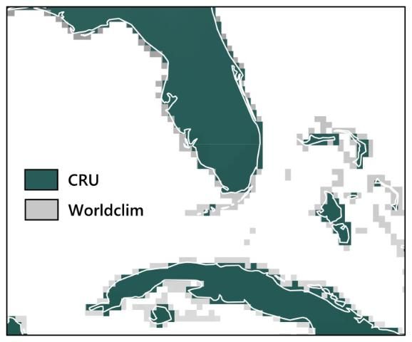
Credit: David Bucklin
For 12 T&E species in Florida, we used a variable selection process to identify which monthly temperature and precipitation variables were most associated with species presences. We then used this set of variables to build models using both CRU and WorldClim datasets.
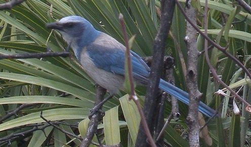
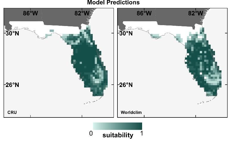
Our results for these 12 species showed that neither model performance nor the prediction maps (for the current time period only) were significantly different depending on which contemporary climate dataset was used (Watling et al. 2014). Figure 4 displays an example of this for the Florida scrub jay (Aphelocoma coerulescens), showing that the broad patterns of the prediction maps using the two different contemporary climate datasets are very similar. Given this result, we found no reason to prefer either of the contemporary climate datasets, concluding that modelers can base their choice of dataset on practical aspects such as availability, spatial resolution, or geographic coverage.
Credit: David Bucklin
Credit: David Bucklin
II. Choice of Future Climate Data
There are many choices to make when choosing future climate data for projecting SDMs, due to the methods climate scientists use to create future climate projections. To predict climate in future decades and centuries, climate scientists employ global climate models (GCMs), which incorporate atmospheric, oceanic, land, sea ice, and other relevant components to simulate global climate patterns. Global climate models are complex and generally produce climate projections at coarse spatial scales (i.e., one projection every 100–200 km; Maraun et al. 2010). There are several dozen GCMs currently in use around the world. In addition, to predict how increased levels of carbon dioxide (CO2) will affect future climate, each GCM can be run using multiple future "scenarios" describing different levels of atmospheric CO2. The combination of all these factors (GCM and CO2 scenario) creates a large number of unique projections of future climate for scientists to choose from.
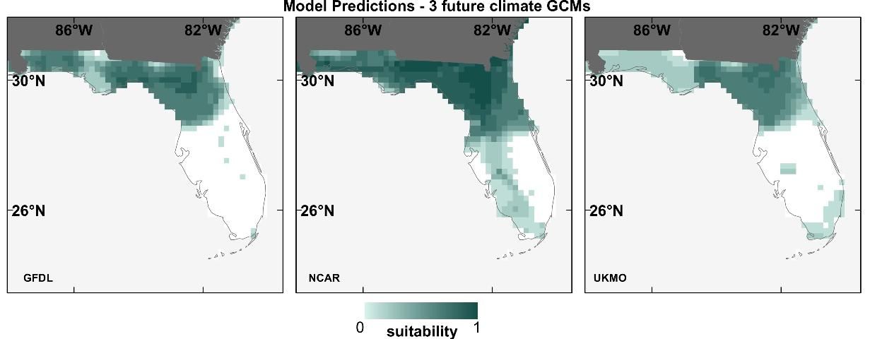
To test how much of an effect GCM choice has on SDMs, we projected the 12 species' SDMs (described in the previous section) into the future (2050) using 3 different GCMs. The results showed that discrepancies can occur among SDM prediction maps using different future GCMs, exemplified for the Florida scrub jay in Figure 5 (Watling et al. 2014). The dissimilarity between SDMs prediction maps using different GCMs (in the future) was higher than that among contemporary prediction maps (Figure 4), indicating less similarity between future GCMs than between contemporary climate datasets.
Credit: David Bucklin
III. Global and Regional Climate Models
Global climate models are useful for projecting climate changes over large areas (e.g., continents), but due to their coarse scale, less useful for representing local or regional climates—the scales at which conservation planning generally takes place. To address this issue, climate scientists often develop complex regional climate models (RCMs) to "downscale" (create higher-resolution) projections from GCMs to much finer scales (e.g., one prediction every 1–50 km), but are limited to one region, using information on factors that influence the climate for that particular region. In contrast to RCMs, another method for downscaling GCMs is "statistical" downscaling, which uses statistical relationships between local and global factors influencing climate to downscale GCM projections (for either one region or the entire world), rather than developing a new climate model (as in RCMs).
To test the effect of RCM vs. statistically downscaled future climate data used for SDMs, we obtained downscaled climate data from both RCM (Stefanova et al. 2012) and statistically-derived (non-RCM) datasets (Tabor and Williams 2010) for 2 GCMs and one climate scenario. Both datasets have ~10-km resolution, and we restricted the analysis to the southeastern United States from 2041–2060. We then created models for 14 of Florida's T&E species and projected them using each of the four different representations of future climate.
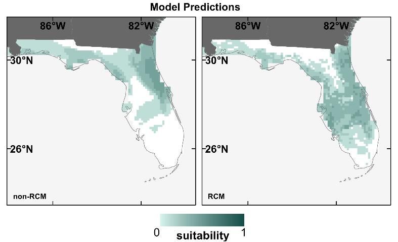
We found that the type of downscaled future climate data (RCM or non-RCM) contributed to moderate to high variation in the SDM prediction maps (Bucklin et al. 2013). For example, for the Everglade snail kite (Rostrhamus sociabilis plumbeus), the SDM prediction map using non-RCM projections predicts loss of suitability throughout much of southern Florida, but one using RCM projections does not (Figure 5). Discrepancies between prediction maps using RCM vs. non-RCM projections were similar to discrepancies among maps using different GCMs projections (as displayed in Figure 4). In general, RCM and non-RCM projections tended to disagree more on future monthly precipitation projections than temperature. Because of the importance of water in many of Florida's eco-systems, RCM projections (which offered more refined precipitation estimates than the non-RCM projections) should offer better SDM predictions for future suitable areas for Florida's wildlife.

Credit: Julio Mulero (https://www.flickr.com/photos/juliom/5431106652), License: CC-BY-NC-ND 2.0
Credit: David Bucklin
IV. Types of Climate Variables
Another choice users of SDMs have to make is the type of climate variables to use in the modeling process. Contemporary climate datasets like CRU and WorldClim are often prepared as monthly averages (e.g., mean temperature in January, mean precipitation in May) or as bioclimate variables, which describe seasonal conditions and/or climate extremes (e.g., maximum temperature of the warmest month, precipitation of the driest season). Bioclimate variables are generally assumed to be more informative for SDMs because certain climatic extremes may be directly limiting to species due to tolerance limits for certain hot, cold, dry, or wet extremes. To test this assumption, we built SDMs using both monthly and bioclimate variables for 12 of Florida's T&E species, and predicted their distributions for the contemporary period only.
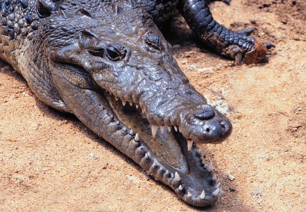
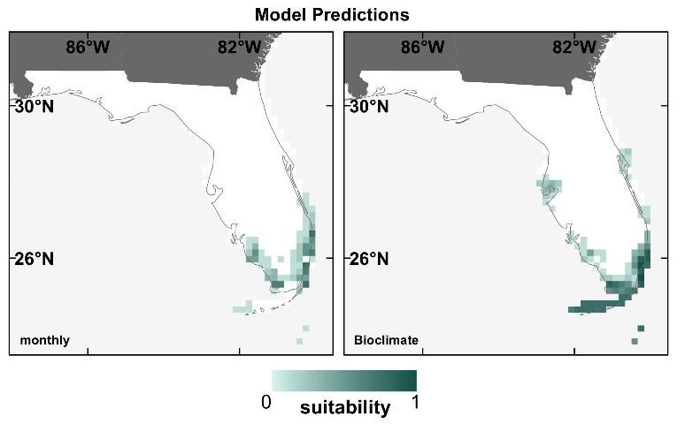
We found no difference in the performance of models built with monthly vs. bioclimate variables (Watling et al. 2012). However, we did note some discrepancy in prediction maps for some species, like the American crocodile (Crocodylus acutus; Figure 8). In addition, for SDMs for species with large ranges, bioclimate variables may be preferable to monthly because of the differences in seasons between the northern and southern hemispheres (for example, the temperature in January represents mid-winter in the North, but mid-summer in the South, and a species occurring in both hemispheres would experience a wide range of conditions in the same calendar month).
Credit: UF/IFAS
Credit: David Bucklin
V. Inclusion of Non-Climate Variables
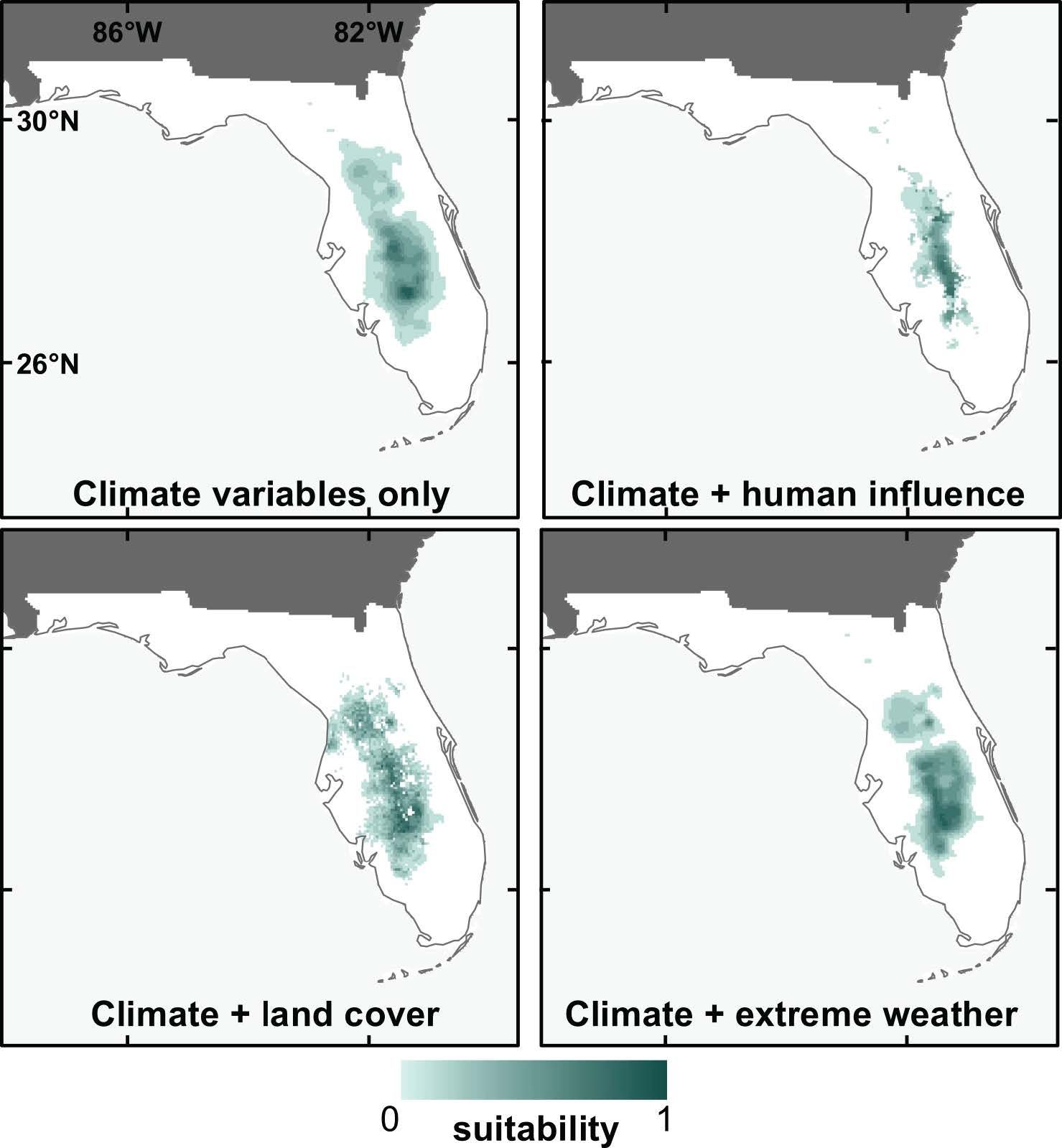
While we know that climate is an important driver of species distributions, we also wanted to know how influential other (non-climate) variables could be in SDMs when used in combination with climate. To test this, we compared models built with climate variables only to those built with climate variables plus variables from several different sets (including land use, human influence, and extreme weather). Models were developed for 14 species that are endemic to Florida, for the contemporary climate period only.
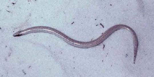
Using metrics that calculate how important individual variables are within a model, we found that climate variables were generally much more important than non-climate variables, regardless of which non-climate variables were combined with them (Bucklin et al. 2015). Performance metrics were not highly variable among any of the models, though we did find that the climate + human-influence models performed significantly better than climate-only models, and that prediction maps from these two models were also the most different from one another. We also found that SDMs including non-climate predictors tended to produce more "refined" prediction maps (smaller suitable areas predicted), as illustrated by prediction maps for the sand skink (Neoseps reynoldsi) in Figure 10.
Credit: USGS
Credit: David Bucklin
VI. Bringing It All Together
To get a unified view of what contributes most to variation in model performance and prediction maps, we conducted a comprehensive "uncertainty analysis" focusing on a number of choices of input data and modeling methods (some also addressed in previous sections), including:
- Contemporary climate dataset (see section I)
- Global Climate Models (GCMs; see section II)
- CO2 emissions scenario
- Algorithm
- Variable selection process (uncorrelated vs. no removal of correlated variables)
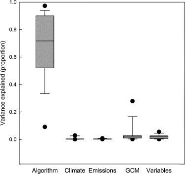
This analysis highlighted each factor's relative contribution to SDM variation (uncertainty). Models were run for 15 species for every combination of the 7 factors, resulting in 48 different models and prediction maps for the contemporary period, and 288 prediction maps (48 × 6 future representations of climate) for the future time period (for each species).
We found that model performance and spatial predictions were most affected by the modeling algorithm applied in the SDM, which strongly outweighed all other factors (Watling et al. 2015). (It is important to note, however, that in many SDM studies, modelers do not use more than one algorithm.) In prediction maps, though, a small amount of variation was also attributable to GCM (for future predictions) and the variable selection process (Figure 12). In addition, variation in the maps was greater in the northern edges of the species' ranges, a direction many of Florida's species are expected to move as the climate warms. These results give strong support for "ensemble" methods for SDMs. Ensemble methods account for uncertainty in a factor by combining models built with several different versions of the factor. For example, SDM users employing ensemble methods could combine prediction maps from multiple algorithms, GCMs, or even species (if they are considering how a group of species may respond to climate change). The ensemble method highlights areas of agreement (and disagreement) between models, giving users a higher level of certainty in their predictions.
Credit: Adapted by authors from Watling et al. (2015)
Conclusion
While SDMs rely on simplified assumptions about species' relationships with their environment, they are still an important tool for understanding how wildlife may respond to environmental changes, and in particular climate change. This document has summarized how certain input data and modelling choices can affect SDM outputs for T&E and endemic species in Florida. Our results regarding the strength of the effect of each choice on model outputs (both model performance metrics and prediction maps), and recommendations regarding each of these choices are given in Table 1.
Results of this work suggest that scientists building SDMs for estimations of wildlife responses to future climate change should focus on using a multiple-algorithm ensemble to project the models for several different representations of future climate. For regional studies, it can be beneficial to use higher-resolution regional climate model (RCM) datasets, when available. In addition, non-climate variables can contribute important information to SDMs, especially when modelers have specific knowledge about how these variables relate to the species, and want more specific range predictions.
With a better understanding of the factors that influence SDM performance and predictions, we can provide better estimates of certainty for SDM predictions. SDMs can generally predict how areas of suitable climate may change for a certain species, but they alone cannot tell us how a certain species will actually respond to changes in climate. In general, a species may respond to climate change in three ways: adjust to new conditions in-place, move to new areas with suitable climates, or go extinct. For some species (e.g., those with ranges restricted to small islands), moving to new areas may not be an option. SDMs can inform conservation planning that aims to allow species to both adapt in place and (for those that are able to) move to newly suitable areas. Such planning will likely minimize loss of biodiversity due to climate change.
References
Bucklin, D.N., J.I. Watling, C. Speroterra, L.A. Brandt, F.J. Mazzotti, and S.S. Romañach. 2013. "Climate downscaling effects on predictive ecological models: a case study for threatened and endangered vertebrates in the southeastern United States." Regional Environmental Change 13(1): 57–68. DOI:10.1007/s10113-012-0389-z
Bucklin, D.N., M. Basille, A.M. Benscoter, L.A. Brandt, F.J. Mazzotti, S.S. Romañach, C. Speroterra, and J.I. Watling. 2015. "Comparing species distribution models constructed with different subsets of environmental predictors." Diversity and Distributions 21: 23-35. DOI: 10.1111/ddi.12247
Maraun, D., F. Wetterhal, A.M. Ireson, R.E Chandler, E.J. Kendon, M. Widmann, et al. 2010. "Precipitation downscaling under climate change: Recent developments to bridge the gap between dynamical models and the end user." Reviews of Geophysics 48(3): RG3003. DOI:10.1029/2009RG000314
Pearson, R.G. and T.P. Dawson. 2003. "Predicting the impacts of climate change on the distribution of species: are bioclimate envelope models useful?" Global Ecology and Biogeography 12(5): 361–371. DOI:10.1046/j.1466-822X.2003.00042.x
Stefanova, L., V. Misra, S. Chan, M. Griffin, J.J. O'Brien, and T.J. Smith III. 2011. "A proxy for high-resolution regional reanalysis for the Southeast United States: assessment of precipitation variability in dynamically downscaled reanalyses." Climate Dynamics 38(11-12): 2449–2466. DOI:10.1007/s00382-011-1230-y
Tabor, K., and J.W. Williams. 2010. "Globally downscaled climate projections for assessing the conservation impacts of climate change." Ecological Applications 20(2): 554–565. DOI:10.1890/09-0173.1
Watling, J.I., S.S. Romañach, D.N. Bucklin, C. Speroterra, L.A. Brandt, L.G. Pearlstine, and F.J. Mazzotti. 2012. "Do bioclimate variables improve performance of climate envelope models?" Ecological Modelling 246: 79–85. DOI:10.1016/j.ecolmodel.2012.07.018
Watling, J.I., R.J Fletcher, C. Speroterra, D.N. Bucklin, L.A. Brandt, S.S. Romañach, L.G. Pearlstine, Y. Escribano, and F.J. Mazzotti. 2014. "Assessing Effects of Variation in Global Climate Data Sets on Spatial Predictions from Climate Envelope Models." Journal of Fish and Wildlife Management 5(1): 14–25. DOI:10.3996/072012-JFWM-056
Watling, J.I., L.A. Brandt, D.N. Bucklin, I. Fujisaki, F.J. Mazzotti, S.S. Romañach, and C. Speroterra. 2015. "Performance metrics and variance partitioning reveal sources of uncertainty in species distribution models." Ecological Modelling 309–310: 48–59. DOI:10.1016/j.ecolmodel.2015.03.017