Introduction
Fertilizer recommendations contain several important factors, including fertilizer form, source, application timing, placement, and irrigation management. Another important part of a fertilizer recommendation is the amount of a particular nutrient to apply. The optimum fertilizer amount is determined from extensive field experimentation conducted for several years, at multiple locations, with several varieties, etc. Although rate is important, rate should be considered as a part of the overall fertilization management program. The important components of a fertilizer recommendation are discussed in Hochmuth and Hanlon (2010a) Principles of Sound Fertilizer Recommendations for Vegetables, available online at https://edis.ifas.ufl.edu/ss527. This EDIS publication focuses on the research principles behind determining the optimum rate of fertilizer, including experimentation and interpreting research results for optimum crop production and quality in conjunction with minimal environmental consequences. We use examples from research with vegetable crops in Florida. How we interpret the results is as important as how we conducted the research.
The target audience for this article includes Extension state specialists, county Extension faculty members, and professionals conducting or working with research in nutrients, agrochemicals, and crop production. The authors assume that the reader has an understanding of basic probability and statistics. Statistical information presented in this publication is intended to demonstrate the process involved in fertilizer experimentation. Explanation of the statistics and their calculations is beyond the scope of this document.
Experimentation
The goal of research on fertilizer rate is to determine the amount of fertilizer needed to achieve a commercial crop yield with sufficient quality that is economically acceptable for the grower. In Florida, these types of studies take a slightly different approach depending on whether soil testing for the nutrient in question is involved. For example, rate studies with nitrogen (N) on sandy soils would not involve soil testing, but rate studies with phosphorus (P) or potassium (K) would. In the case of N on sandy soils, the researcher assumes there is minimal N supplied from the soil that would satisfy the crop nutrient requirement. In the case of P or K, a properly calibrated soil test will reveal if a response (yield and fruit quality) to the nutrient is likely or not. Rate studies are best conducted on soils low in the particular nutrient so that maximum crop response is likely and that response can be modeled.
Proper experimental design and statistical data analyses are critical to interpretation of the results. Research begins with a hypothesis or a set of hypotheses. One possible hypothesis may be that there will be no effect on yield associated with N fertilization. This hypothesis, called the null hypothesis, is evaluated with an experiment to test crop yield response against a range of N rates in a field likely to produce a large response to the addition of N fertilizer.
The researcher applies a range of fertilizer rates thought to capture the likely extent of possible crop yield responses. A zero-fertilizer treatment is always included. Crop response without an actual fertilizer application demonstrates and measures the soil-supplied effects, if any. In some cases, sufficient nutrients, or at least a low portion of the crop nutrient requirement, may come from the soil, while in other cases, nutrients may come from the irrigation water.
The researcher may decide to divide the total seasonal amount of fertilizer into split-applications, following what would likely be a recommended practice for the crop being studied. Multiple applications avoid potential large losses of fertilizer because of rainfall events, especially for nutrients that are mobile in the soil. Typically, all treatment rates are handled similarly for timing and placement of the fertilizer to minimize any confounding effects with rate.
During the growing season, the researcher may sample the plant for nutrient concentrations, using whole dried leaves and/or fresh petiole sap. These samples will help the researcher prove the response in yield was related to the plant's nutrient status. Typically, soil samples are not used because there is a chance of including a fertilizer particle in the sample, or there may be questions of where to sample if the fertilizer is applied by banding or through a drip tape. Photographs taken during the season are useful for documenting both growth and potential plant deficiency symptoms.
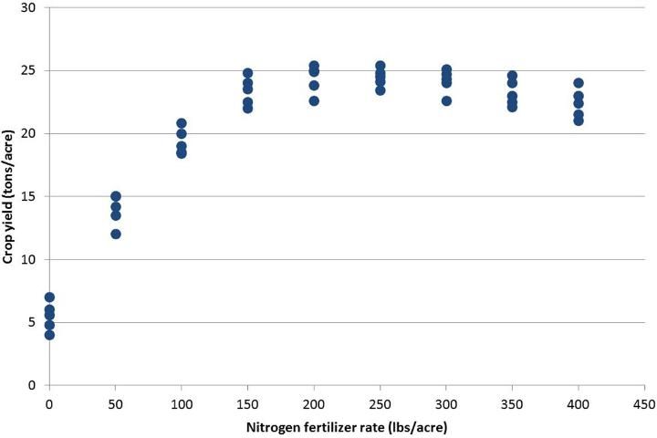
The crop response of interest, typically marketable yield, is measured at the appropriate harvest time(s). For vegetables, the fruits are evaluated according to USDA grade standards to detect any effects of fertilization on fruit quality (size, color, sugar content, etc.). Yields are expressed in the prevailing commercial units per area of production (e.g., 28-lb boxes/acre, 42-lb crates/acre, bushels/acre, tons/acre, etc.). The raw data should be plotted in a scatter diagram (Figure 1) to gain insight into the type and magnitude of response. Plotting the raw data allows the researcher to inspect for apparent atypical data points that may illustrate errors somewhere in the data entry process.
Once the data have been collected and inspected, they are analyzed statistically with analysis of variance (ANOVA). Did fertilization have a significant effect on yield? ANOVA is particularly useful in cases where a researcher might be evaluating the effect of fertilizer rate across several varieties of crop. Here, the researcher is interested in whether varieties differed in response to fertilizer, which will be exposed through a significant interaction term in the ANOVA source table. If the fertilizer treatment effect was significant, then the researcher will want to graphically present the results with a mathematical equation sometimes called a "model."
In fertilizer rate experiments, the rate of fertilizer is referred to as a continuous variable because there are many possible rates in addition to the ones the researcher selected to use in the experiment. Using ANOVA, especially if the experiment had the treatments arranged in a factorial arrangement, is a good approach to test for treatment effects and interactions. Fertilizer rate main effects can be subjected to polynomial contrasts, a statistical method to determine if there are linear or quadratic components in the overall response. Then regression methods can be applied to the continuous variable to develop an equation that explains the significant trend in response (see the section below about models).
The ANOVA statistics for a randomized complete-block N experimental design (data in Figure 1) with five replications and nine N rates indicate that one or more N rate treatments were statistically different from the others (Table 1). In this case, our null hypothesis would have been rejected. Since ANOVA tables contain estimates of several variance components, these tables should be included in research manuscripts but are seldom included. For example, other researchers may be able to use this information when summarizing numerous, similar studies. While simply reporting means and treatment effects is good for a simple research report or presentation, this method does not contain measures of variance, and the ANOVA table does.
Treatment Significance
Researchers cannot study every possible experimental treatment (rate) or combinations of treatments. In addition, there is natural variation in the field where the research will be conducted. The field may have variations in organic matter, soil pH, or moisture, all of which may lead to variations in yield response having nothing to do with the N treatment(s). Therefore, the notion of probability comes into play. What are the chances that the observed differences in yield are because of natural variation from plot to plot? This inherent variability is where statistical analysis of the data helps to sort out the differences most likely caused by treatment (N fertilization) from the so-called "noise" or random error in the production system. If we repeat the application of treatments, called replication, we can estimate the relative amount of natural variation. Experiments should always include replication as part of a properly designed experiment, one that would pass a peer-review process. Analysis of variance is the mathematical tool we use for this analysis, and with this statistical tool we can test the relative proportion of the variation due to treatment effects against the variation due to chance.
The generally accepted probability level of 0.05 (5%) is used in agricultural research as the probability that there could be a real difference when ANOVA indicates no such difference. This probability level is the level of error that scientists are willing to accept. In other words, a real difference is so rare that it is of minimal practical concern. If the experiment were repeated 20 times, there would be a 1 in 20 chance that our hypothesis would not be rejected. Said another way, if the ANOVA indicates a difference between one or more treatments, we are 95% certain that this difference is a real effect. We call these differences "significant" differences. If ANOVA detects significant differences among treatment means, then we reject our null hypothesis.
In the "real world," finding no significant differences has two major implications. First, it means that farmers should not be interested in spending extra money each year (for "insurance" applications) just to gain the rare possibility of a real crop response. These unjustified expenses would reduce profitability. The second implication is the potential negative impacts on the environment when a rate of fertilization is applied to the crop when not needed.
One common misinterpretation about treatment differences needs clarification. For example, assume an experiment was conducted to test the effect of N rate on tomato yield and the ANOVA found no significant difference between the grower rate and the recommended (lower) rate at the 5% probability level. This finding means that there is such a rare chance of a real treatment difference occurring that we can be confident the grower can reduce the commercial fertilizer rate. The actual means may be 2,950 and 2,920 boxes/acre for the grower and recommended rates, respectively. An argument could be made to someone without knowledge in statistics that the 30 boxes/acre "difference" is "worth" $600 (30 boxes at $20/box) and that amount will more than pay for the added fertilizer with the grower rate. This conclusion is erroneous because the ANOVA indicated no significant difference between the two treatment means. Therefore, the appropriate representation of the response to fertilizer is the average of the two means (i. e., 2,935 boxes per acre). Said another way, other factors on the farm impact yield more than fertilizer rate.
A more complex experiment may be to test the response of two cultivars to N rate. Here, ANOVA is used to test the significance of the main effect of N rate, the main effect of cultivar, and the interaction in the response of cultivar to N rate. There are two outcomes depending on whether or not there is an interaction of N rate and cultivar (i. e., that the cultivars differed in their response to N rate). If there was no interaction, then the response to N can be averaged using both cultivar means. If an interaction is observed, then each cultivar response must be evaluated separately.
Mathematical Descriptions of the Response (Models)
In statistical terms, fertilizer rate research employs various levels of a quantitative variable, the amount of fertilizer. If the ANOVA indicates a significant N treatment effect, as in Table 1, then the researcher will wish to further evaluate the response with the development of the mathematical model. Responses to a quantitative variable can be statistically inspected along the full range of the levels of the variable, and the responses to rates in between those actually applied in the field can be calculated. In most fertilizer experiments, a set of 4 to 5 levels of fertilizer plus a zero-fertilizer control is sufficient for most models. The results can be presented graphically by an equation or model. The model can be used to predict results if a second experiment similar to the first were conducted. Models are typically developed with regression analyses.
Various models can be fit to a set of data to explain the responses. A linear model might explain a response that continues upward or downward in a straight line within the range of tested fertilizer rates. A linear response may mean the chosen range of treatments was insufficient to determine the maximum (or minimum) yield. A quadratic response is typical of crop yield in which the response increases with fertilizer rate to a point where yield approaches a maximum but then might decrease at higher rates. In other words, there is a point at which increased fertilizer does not result in a significant increase in yield. Quadratic models also typically have a linear component, meaning that as fertilizer rates increase from low to medium rates the yield also increases. At a certain point, the rate of yield increase starts to stabilize or decline.
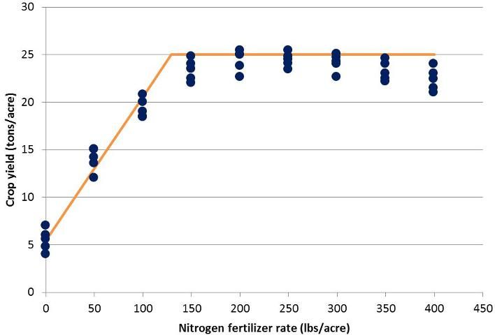
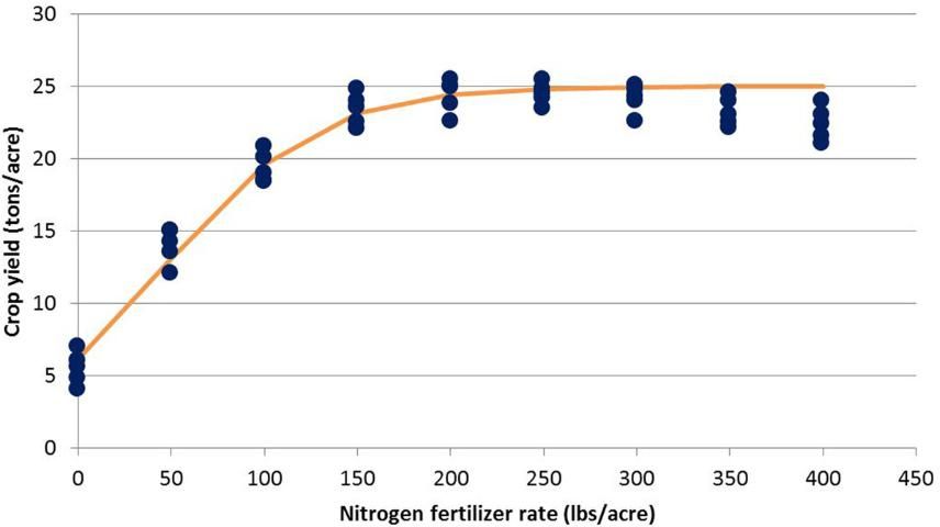
Linear and quadratic models are the simplest equations to use for explaining crop responses to fertilizer, and they have served scientists well as long as the main interest in the research was maximizing yield. However, today there are other goals in fertilizer research, including economics and environmental issues. Several researchers have explored different models for explaining crop responses to fertilizer (see the articles in the list of references at the end of this publication). Studies have found that the quadratic model leads to overestimation of fertilizer recommendations derived from responses to fertilizer (Cerrato and Blackmer 1987; Hochmuth et al. 1993a; 1993b; 1996; Willcutts et al. 1998). If the goal of the research was to select a fertilizer rate to be used as a recommended practice, then the quadratic model will usually predict a greater fertilizer need if the maximum point from the model is taken as the putative recommendation. The maximum yield mean is not always significantly different from one or more means resulting from lesser fertilizer rates. If we inspect the plot of data in Figure 1, we might predict that there is little difference in yields among the fertilizer rates from 150 lb/acre or greater. Other models have been identified that result in a lower, but agronomically acceptable, recommended fertilizer rate, saving fertilizer expense and reducing the risk of excessive fertilizer applications that might endanger the environment.These models include the logistic and the linear-plateau models. Using the data in Figure 1, these three models are illustrated in Figure 2, Figure 3, and Figure 4.
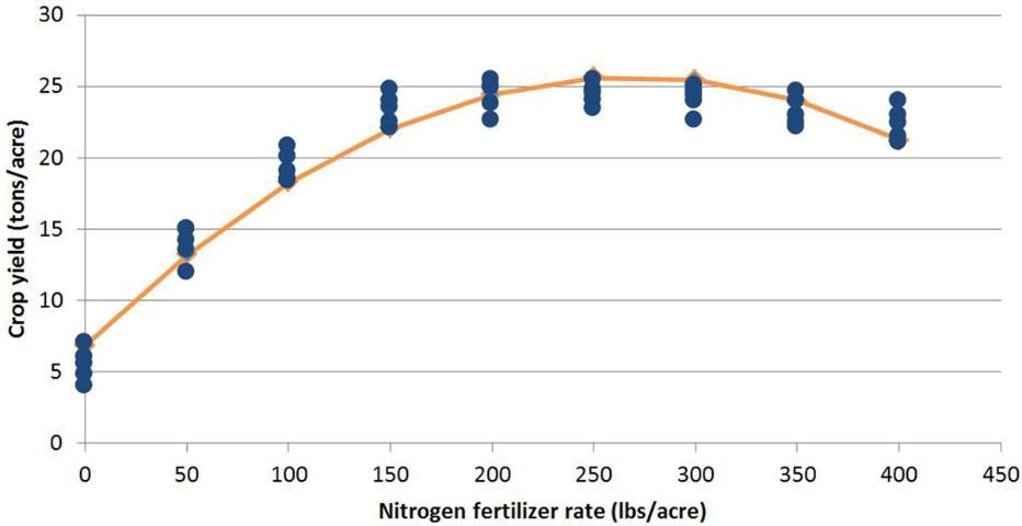
Researchers use statistics and mathematical models as tools to help explain crop response to fertilizer. We should keep in mind that models are tools, and we should exercise care in their use. The three models depicted here have been fit to the same data set first presented in Figure 1. We know from the ANOVA that crop responded to fertilizer in a significant way, but ANOVA does not identify which fertilizer rate was superior. However, each model tells a different story about the response, if we focus only on a model's parameters. The most commonly used model in agronomic and horticultural crop response research is the quadratic model (Figure 2). The quadratic model is easy to derive by computer statistical packages, and most researchers are familiar with it from their graduate training. Also, the quadratic model is easily differentiated to show a peak yield and its associated fertilizer rate.
The problem with relying solely on the quadratic model occurs on inspection of the mean yields versus fertilizer rate. It could be argued and can be shown by orthogonal contrasts that there is a leveling-off of yield. Further, this leveling-off occurs at a fertilizer rate less than the peak yield derived from the quadratic model. In an environmentally aware society, perhaps researchers should not simply interpret the quadratic model maximum as the putative fertilizer recommendation for rate.
An optional model being used by scientists more frequently is the linear-plateau model (Figure 3). This model also yields critical model parameters, the plateau and the shoulder point. The plateau illustrates the notion that there is a leveling-off of crop yield response to fertilizer. However, the linear-plateau model shoulder point could be argued to be too conservative as a putative fertilizer recommendation.
Several recent research studies with vegetables in Florida have illustrated the challenges with the quadratic and linear-plateau models if used alone (Hochmuth et al. 1993a; 1993b). These researchers proposed using the midpoint between the shoulder point in the linear-plateau model and the peak in the quadratic model as a putative recommended rate. For our data, this midpoint would be 200 lbs/acre of N fertilizer.
A third model (Figure 4), the logistic model, has been proposed by Overman and colleagues in studies with agronomic and vegetable crops (Overman et al. 1990; 1992; 1993; Willcutts et al. 1998). The logistic model is a reasonable compromise between the quadratic and linear-plateau models. First, this model illustrates the law of diminishing returns. As the rate of nutrient is increased, the yield increases until an area of diminishing returns. Second, the slope of this model is not unusually steep. Third, the function does not pass through the origin; therefore, no negative yields would be predicted, nor are zero yields predicted with zero fertilizer added. Thus, this model accounts for native soil fertility. These attributes make the logistic model particularly useful for making fertilizer recommendations that avoid under- or over-fertilization.
In typical agronomic or horticultural crop yield response data, rarely are yields between 90% and 100% of maximum declared significantly (probability = 5%) different. Selecting 95% of maximum yield to derive the putative recommended fertilizer rate would be a conservative approach to ensure a most suitable fertilizer rate that would result in profitable yields with due diligence in considering the risk to the environment.
Using the data set above, the considerations for a fertilizer recommendation would include the following:
- Quadratic model: The predicted peak crop response is 25.6 tons/acre with 270 lbs/acre N.
- Linear-plateau model: The plateau yield is 25 tons/acre and the shoulder point fertilizer rate is 129 lbs/acre N.
- Logistic model: 95% maximum yield (25 tons/acre) occurs at 168 lbs/acre N, and 97% maximum occurs with 190 lbs/acre.
The list above shows that, depending on the level of conservatism applied, the putative fertilizer recommendation could range from 129 to 270 lbs/acre N, a 100% difference. Selecting the midpoint between the shoulder point of the linear-plateau and the peak of the quadratic model or taking a conservative 97% maximum yield with the logistic model yields similar results. This analysis yields a putative fertilizer recommendation of approximately 200 lbs/acre N. Choosing 200 lbs/acre instead of 270 lbs/acre as the recommendation results in no sacrifice in yield but saves 70 lbs/acre of fertilizer. This is both an economic savings as well as a real removal of nutrient load from the environment.
An Example from Actual Research in Florida
The figures above are helpful to illustrate the principles of research and data presentation. What about actual data from Florida? There have been several research studies conducted with vegetables in Florida evaluating yield and fruit quality responses to fertilization with various models. One such study was conducted with watermelon (Figure 5).
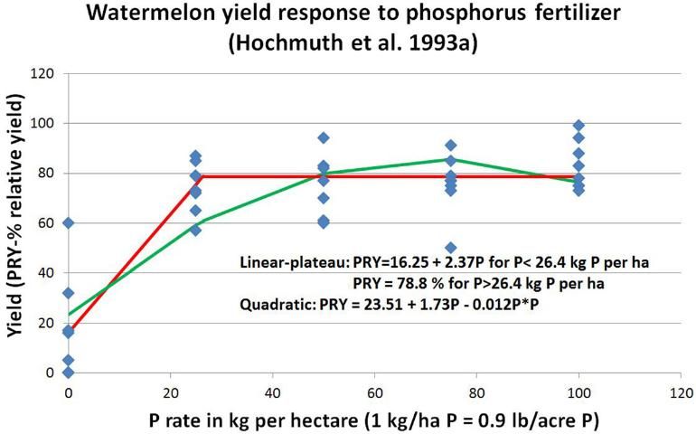
In the watermelon study, the shoulder point for the linear-plateau occurred at 26.4 kg ha-1 P or approximately 53 lbs/acre P2O5. The quadratic model maximum yield occurs with 75 kg ha- 1 P or 150 lbs/acre P2O5. Statistical analysis (ANOVA and contrasts) of the data showed no significant difference in yield from 50 to 200 lbs/acre P2O5. The shoulder value is on the verge of steep yield reduction with less than 53 lbs/acre P2O5, but the quadratic maximum yield occurred with excessive fertilization. The authors of this research paper proposed using the midpoint between the linear-plateau shoulder point and the quadratic maximum point as a reasonable compromise fertilization recommendation. In this case, the recommendation could be about 100 lbs/acre P2O5. This recommendation would result in considerable savings in P fertilizer compared to the current recommendation of 160 lbs/acre P2O5 for soils with low or very low Mehlich-1 P concentration.
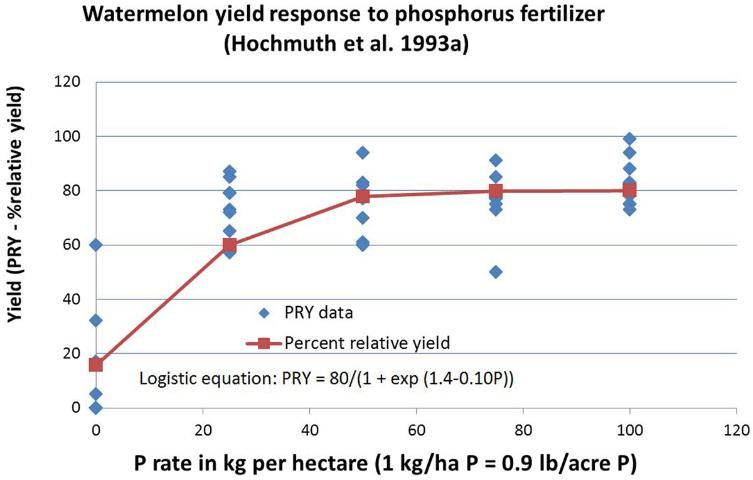
Using the logistic model (Figure 6) yields a conclusion similar to using the midpoint between the quadratic maximum and the shoulder point of the linear-plateau model. Using 97% of the maximum yield would result in a fertilizer recommendation of approximately 55 kg/ha P or 115 lbs/acre P2O5.
There are additional reasons (beyond environmental) for making recommendations closer to the conservative side of the response curve. There are numerous research reports about excessive fertilization, especially N, having a negative impact on yield and fruit quality. The slight depression in yield at excessive fertilizer rates, coupled with the cost of the extra fertilizer, may lead to significant reductions in farm profits. Furthermore, research results have been published in the peer-reviewed literature documenting reductions in fruit and vegetable quality parameters by excessive fertilization (Hochmuth et al. 1996; 1999).
Some Comments about Percent Relative Yield (RY)
Crop responses are an integration of many different aspects of the entire production system to which the crop is exposed. Research completed during one season is affected by the crop integration process during that entire season, as well as some antecedent contributors, such as nitrogen mineralization from crop residue or soil organic matter. The problem with crop responses associated with different experiments conducted by separate research groups, and often for different purposes, is that the observed crop yields in each of the individual experiments will display variation. Plotting all the data from many experiments in the original units yields a scatter-graph that renders a general interpretation very difficult. One method that can be used to get a sense of the crop response to fertilization across numerous studies is the percent relative yield. The highest yield obtained in that particular experiment in that particular season is assigned as 100% relative yield. All other yields are calculated by dividing the observed yield by the highest actual yield and are expressed as a percentage.
Transforming the original data in this manner adds to the flexibility of looking at the relative yields, which have been brought to a common scale. The value of this type of transformation is that researchers get a sense of how that particular crop responded to fertilizer additions throughout many seasons, locations, and production practices. Relative yield should be used with caution to avoid putting too much emphasis on this data transformation and resulting graph alone. For example, using all the RY values from several experiments for subsequent regression can be quite misleading, especially for calculating actual yields. However, noticing that the variability among all responses decreases after fertilizer rate exceeds a certain range becomes quite obvious.
There are a number of assumptions built into this transformation process. The primary assumption is that most or all of the response that we note in an RY graph is due to fertilizer. There have been extensive arguments both for and against making this assumption. In summarizing this debate, Black (1992) indicates that the assumption can be considered valid when using the RY plot to explore variation across the years, seasons, and other production practices. Black cautions the reader to avoid additional statistical evaluations of the RY plot due in part to its statistical characteristics (not normally distributed) and the true shape of the yield response to added fertilizer is site-specific. The RY plot generalizes the site-specific variations in nature of soil, fertilizer, climate, and plant interactions. Problems with this generalization are avoided if the RY plot is not used for subsequent regression analysis involving actual yields and further interpretation.
For those who are interested in statistics, this type of transformation also has a weighting factor based upon the selection of the maximum yield. Again, this weighting factor makes the assumptions above and is reduced to insignificance by using the RY plot on a visual basis only and not trying to further statistically analyze the regression by other means. Black (1992) states that while these objections are worthy of note, the RY plot can be a useful tool in fertilizer research.
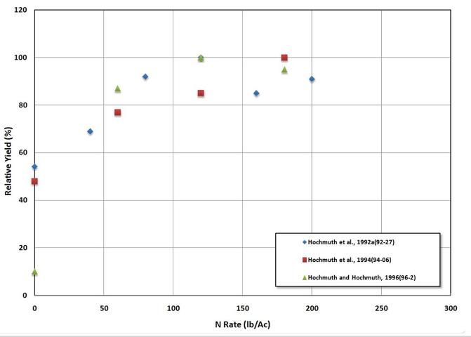
To further illustrate the usefulness of the percent relative yield approach, watermelon yield is plotted in Figure 7. Note that the yields increase in all experiments and then tend to level off somewhere between 100 and 200 lbs/acre N. The current UF/IFAS N recommendation is 150 lbs/acre N. While this graph was not used to set the UF/IFAS recommendation, the graph indicates that the recommendation is reasonable and supported by research.
Summary
Crop fertilizer response research should be carefully conducted to account for the economics to the grower and protection of the environment from nutrient losses due to excessive fertilization. There are several mathematical models to describe crop yield response to fertilizer, and these models should be employed with caution. Using a single model to explain crop response may not account for economics and potential environmental impact together. This problem is evident with the quadratic and linear-plateau models. Incorporating both models in the data response interpretation and calculating the midpoint as we have demonstrated above will consider both goals. The logistic model appears to be the best single model at considering both economics and environmental goals. There is increasing accumulation of research documenting the impacts of over-fertilization on yield and quality, thus reducing profits. Added to these reasons is the need to protect the environment from nutrient pollution related to farming activities. It becomes evident that how research is conducted and how the data are analyzed and interpreted are critical to developing an informed fertilizer recommendation.
References
Black, C. A. 1992. Soil Fertility Evaluation and Control. Boca Raton, FL: Lewis Publishers.
Bullock, D. G., and D. S. Bullock. 1994. "Quadratic and Quadratic-plus-plateau Models for Predicting Optimal Nitrogen Rate of Corn: A Comparison." Agron. J. 86:191-5.
Cerrato, M. E., and A. M. Blackmer. 1987. "Comparison of Models for Describing Corn Yield Response to Nitrogen Fertilizer." Agron. J. 82:138-43.
Dahnke, W. C., and R. A. Olson. 1990. "Soil Test Correlation, Calibration, and Recommendation." In Soil Testing and Plant Analysis, 3rd edition, edited by R. L. Westerman, 45-71. Madison, WI: Soil Sci. Soc. Amer.
Hochmuth, G. J., E. E. Albregts, C. C. Chandler, J. Cornell, and J. Harrison. 1996. "Nitrogen Fertigation Requirements of Drip-irrigated Strawberries." J. Amer. Soc. Hort. Sci. 121:660-5.
Hochmuth, G. J., J. K. Brecht, and M. J. Bassett. 1999. "N Fertilization to Maximize Carrot Yield and Quality on a Sandy Soil." HortScience 34(4): 641-5.
Hochmuth, G. J., J. Brecht, and M. J. Bassett. 2006. "Fresh-Market Carrot Yield and Quality Responses to K Fertilization of a Sandy Soil Validated by Mehlich-1 Soil Test." HortTechnology 16:270-6.
Hochmuth, G. J., and E. A. Hanlon. 2010a. Principles of Sound Fertilizer Recommendations. SL315. Gainesville: University of Florida Institute of Food and Agricultural Sciences. https://edis.ifas.ufl.edu/ss527
Hochmuth, G. J., and E. A. Hanlon. 2010b. Summary of N, P, and K Research with Watermelon in Florida. SL325. Gainesville: University of Florida Institute of Food and Agricultural Sciences. https://edis.ifas.ufl.edu/cv232
Hochmuth, G. J., E. A. Hanlon, and J. Cornell. 1993a. "Watermelon Phosphorus Requirements in Soils with Low Mehlich-1 Extractable Phosphorus." HortScience 28:630-2.
Hochmuth, G. J., R. C. Hochmuth, M. E. Donley, and E. A. Hanlon. 1993b. "Eggplant Yield in Response to Potassium Fertilization on Sandy Soil." HortScience 28:1002-5.
Nelson, L. A., and R. L. Anderson. 1977. "Partitioning of Soil-test Response Probability." In Soil Testing: Correlation and Interpreting the Analytical Results, spec. publ. 29, edited by T.R. Peck, J.T. Cope, and D.A. Whitney, 19-38. Madison, WI: Am. Soc. Agron.
Overman, A. R., F. G. Martin, and S. R. Wilkinson. 1990. "A Logistic Equation for Yield Response of Forage Grass to Nitrogen." Commun. Soil. Sci. Plant Anal. 21:595-609.
Overman, A. R., M. A. Sanderson, and R. M. Jones. 1993. "Logistic Response of Bermudagrass and Bunchgrass Cultivars to Applied Nitrogen." Agron. J. 85:541-5.
Overman, A. R., and S. R. Wilkinson. 1992. "Model Evaluation for Perennial Grasses in the Southern United States." Agron. J. 84:523-9.
Willcutts, J. F., A. R. Overman, G. J. Hochmuth, D. J. Cantliffe, and P. Soundy. 1998. "A Comparison of Three Mathematical Models of Response to Applied Nitrogen: A Case Study Using Lettuce." HortScience 33:833-6.