Mapping the US Census Data Using the TIGER/Line Shapefiles
Young Gu Her and Ziwen Yu
Introduction
Geospatial data are critical to understanding the spatial variations of a variable of interest. The US Census TIGER/Line Shapefiles have been a useful and reliable source of demographic and geographic information, including administrative boundaries, population and housing unit counts, road lines, address information, and water features. Such information helps users understand and identify target stakeholders and areas. It is critical to develop Extension and research programs that can help users make informed decisions at the local, state, and national levels using the spatial information. This article introduces the TIGER/Line Shapefile datasets and demonstrates how we can extract and map spatial information from the US Census data using the shapefiles. This publication will help Extension agents and decision-makers to map and analyze the demographic and geographic data provided by the US Census survey data and the TIGER/Line Shapefiles using commonly available tools and software.
What is a shapefile?
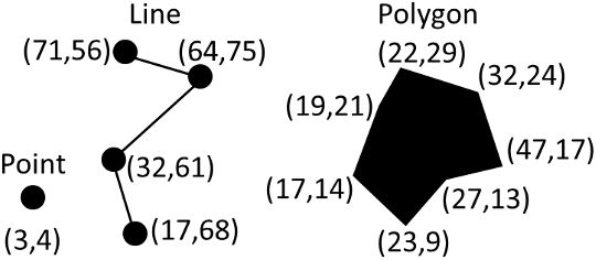
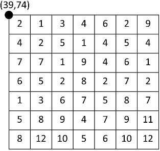
A shapefile is a set of associated files that contain geospatial data and information (e.g., location, shape, and map projection) of spatial objects such as buildings (points or polygons), roads (lines or polygons), and areas (polygons) (Figure 1). Here, “shape” means the external boundary or outline of an object, and map projection is a way to represent the three-dimensional Earth surface on a two-dimensional plane or paper. The Environmental Systems Research Institute (ESRI) first created the shapefile format for use in its geographic information system (GIS) software, ArcGIS® (previously ArcInfo® and ArcView®), but the shapefiles work with other GIS software such as QGIS (Quantum GIS) (Flenniken et al. 2020) as well. In a shapefile, spatial objects are depicted as vectors, which can represent points (e.g., a point of interest such as a landmark and house), lines (e.g., roads), or polygons (e.g., boundaries of farms and counties) with vertices and paths (Figure 1). The vertices (e.g., points in Figure 1) and paths (e.g., lines in Figure 1) contain spatial information such as location (e.g., latitude and longitude). Nonspatial information associated with these vector objects, such as population size, density, and characteristics, are called attributes. Shapefiles are commonly used when representing spatial information of objects and storing their nonspatial attributes. A raster (or grid) is another common format of spatial data. In a grid, square cells are divided into rows and columns, and each cell has a value that represents the characteristics of the corresponding location, such as elevation and land use (Figure 2). Grid files are good at storing information that can be represented with regularly spaced data, such as an array of pixels of a photo and remotely sensed image (Figure 2). Grid formats are commonly used to represent continuous surface (i.e., elevations [topography], soil characteristics, land uses) and weather variables (e.g., air temperature and precipitation) across a region.
Credit: Young Gu Her and Ziwen Yu, UF/IFAS
Credit: Young Gu Her and Ziwen Yu, UF/IFAS
What are TIGER/Line Shapefiles?
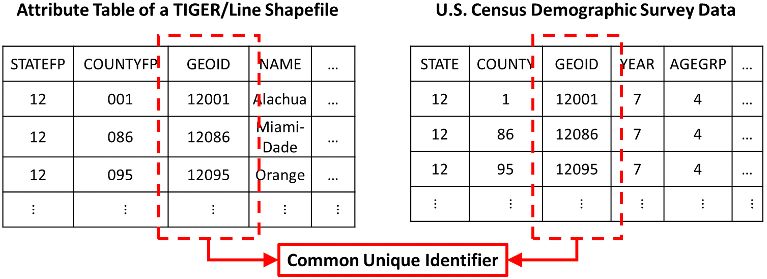
The US Census Bureau uses the TIGER/Line Shapefiles to store geographic and cartographic information from the US Census Bureau’s Master Address File/Topologically Integrated Geographic Encoding and Referencing (MAF/TIGER) database. “MAF/TIGER is the Census Bureau’s geographic database. MAF is a complete inventory of housing units and business locations in the United States, and it was originally built from the US Postal Service’s Delivery Sequence File of all residential addresses. MAF/TIGER refers to the coupling of the MAF with the TIGER spatial database” (DiBiase 2014). The TIGER/Line Shapefiles do not include demographic data but geographic entity codes (GEOIDs), which can serve as geospatial identifiers of the Census Bureau’s demographic data, linking the two databases (Figure 3). The TIGER/Line Shapefiles contain geospatial information for the 50 states, the District of Columbia, Puerto Rico, American Samoa, the Commonwealth of the Northern Mariana Islands, Guam, and the United States Virgin Islands. This information includes the boundaries (areas; polygons) of states, counties, and census blocks, roads and hydrography (streamlines; lines), and landmarks (e.g., schools, airports, and parks; points) (Table 1). In addition to the TIGER/Line Shapefiles, “the Census Bureau creates additional shapefiles and geodatabases that include demographic data. These are as-is products and are created by Census Bureau staff as time permits. All shapefiles and geodatabases with demographic data are available at: https://www.census.gov/programs-surveys/geography.html.” The details of the methods used to estimate populations for the US Census data can be found from the US Census (2020a).
Credit: Young Gu Her and Ziwen Yu, UF/IFAS
Table 1. Layer types of the TIGER/Line Shapefiles.
Relationship between the TIGER/Line Shapefiles and Census Statistical Data
The TIGER/Line Shapefiles contain a standard geographic identifier (GEOIDs) for each spatial object. The object links to GEOIDs of each demographic record from censuses and surveys, including the Decennial Census, Economic Census, American Community Survey, and the Population Estimates Program (Figure 3). The US Census data are not prepared in the shapefile format; therefore, it is necessary to link the census data to a geospatial layer including the TIGER/Line Shapefiles to map interesting demographic variables such as populations, ages, genders, and races. We can join data from many of the Census Bureau’s surveys and censuses, which are available in American FactFinder (US Census 2020b), to spatial objects of the TIGER/Line Shapefiles using GIS software such as ArcGIS® and QGIS to see the spatial distributions of a variable of interest. For instance, we can map the roads and water bodies on the top of county boundaries, count the number of people in age groups in the counties of interest, and map population compositions at the county level. Such examples are demonstrated later in this article.
Tools Available for Mapping the Data
The TIGER/Line Shapefiles data can be viewed using multiple tools with different functionalities. To map the vector features on a map and to view the labels, various districts, roads, and some specific areas, the online tool, TIGERweb (https://tigerweb.geo.census.gov/tigerwebmain/TIGERweb_main.html), would be the most convenient interface. It is supported by the US Census Bureau. It also contains the types of features used in the US Census Bureau's surveys and stored in their digital mapping database. To further analyze the geospatial distribution of certain attributes found in the TIGER/Line Shapefiles data, offline tools are desired for their full functionalities. The offline or standalone GIS tools include, but are not limited to, ArcGIS® (by ESRI), MapInfo® (by Pitney Bowes Software), and QGIS (Open Source GIS licensed under the GNU General Public Licenses). In this article, QGIS was selected as a GIS tool to demonstrate the association between TIGER/Line Shapefiles vector features and US Census data, because QGIS is a free open source software that anyone can use and modify (Flenniken et al. 2020).
Examples
This article introduces three case studies to demonstrate how to use the TIGER/Line Shapefiles with the US Census data: mapping counties, roads, and water bodies; counting the number of people in an age group; and mapping population compositions by race and ethnicity.
To obtain the software and data required for these examples, follow the steps below.
- Download and install QGIS software.
- Download the installation file of a QGIS version that is suitable for the operating system (e.g., Windows, iOS, and Linux) of your computer: https://qgis.org/en/site/.
- Install QGIS on your computer by running the downloaded installation file. QGIS 3.10.10 was used for the examples in this article.
- Download the county boundary shapefile (polygons) from the TIGER/Line Shapefiles.
- Go to https://www.census.gov/cgi-bin/geo/shapefiles/index.php.
- Select “2019” from the “Select year” dropdown menu and “Counties (and equivalent)” from the “Select a layer type” dropdown menu. Click the “Submit” button to download a ZIP file, “tl_2019_us_county.zip.”
- Unzip (or extract) the downloaded file.
- Download the road shapefile (line) from the TIGER/Line Shapefiles.
- Go to https://www.census.gov/cgi-bin/geo/shapefiles/index.php.
- Select “Roads” from the “Select a layer type” dropdown menu, then click the “Submit” button to move to the next webpage (https://www.census.gov/cgi-bin/geo/shapefiles/index.php?year=2019&layergroup=Roads).
- On the next webpage, select “Florida” from the “Select a State” dropdown menu under “Primary and Secondary Roads” and click the “Submit” button to download a ZIP file, “tl_2019_12_prisecroads.zip.”
- Unzip the downloaded file.
- Download the water (e.g., waterbody and water boundary lines) area shapefile (polygons and lines) from the TIGER/Line Shapefiles.
- Go to https://www.census.gov/cgi-bin/geo/shapefiles/index.php.
- Select “Water” from the “Select a layer type” dropdown menu and then click the “Submit” button to move to the next webpage (https://www.census.gov/cgi-bin/geo/shapefiles/index.php?year=2019&layergroup=Water).
- On the next webpage, select “Florida” from the “Select a State” dropdown menu.
- Select “Alachua County” from the “Select a County” dropdown menu and click the “Download” button to download a ZIP file, “tl_2019_12001_areawater.zip.”
- Unzip the downloaded file.
- Access the population data with age attributes from the US Census for Florida.
- Go to https://www.census.gov/data/tables/time-series/demo/popest/2010s-counties-detail.html.
- Select “Florida” under “Annual County and Resident Population Estimates by Selected Age Groups and Sex: April 1, 2010 to July 1, 2019 (CC-EST2019-AGESEX)” to download the resident population estimates by selected age groups, “cc-est2019-agesex-12.csv.” Details of the dataset can be found at https://www2.census.gov/programs-surveys/popest/technical-documentation/file-layouts/2010-2019/cc-est2019-agesex.pdf.
- Select “Florida” under “Annual County Resident Population Estimates by Age, Sex, Race, and Hispanic Origin: April 1, 2010 to July 1, 2019 (CC-EST2019-ALLDATA)” to download the resident population estimates by races, “cc-est2019-alldata-12.csv.”
To load all the shapefiles into QGIS, you need to run QGIS and create a new project. Flenniken et al. (2020) provide a useful primer for those who are unfamiliar with QGIS. More detailed instructions on using QGIS can be found in a QGIS user guide and manual (https://docs.qgis.org/3.10/en/docs/training_manual/index.html).
Example 1: Mapping Counties, Roads, and Waterbodies
The first example is intended to demonstrate how to compile different spatial objects in multiple layers (or TIGER/Line Shapefiles) in a QGIS project.
- Open the downloaded shapefiles, including the county boundary shapefile, the road shapefile, and the water area shapefile, in QGIS.
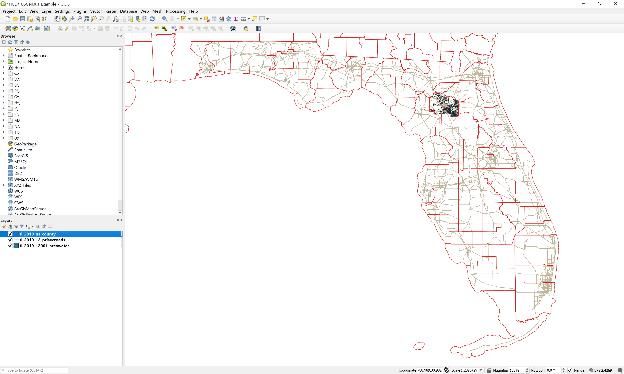
- Map all their features at the state level (primary and secondary roads; Figure 4), then to Gainesville, FL (waterbodies and linear water; Figure 5).
Credit: Young Gu Her and Ziwen Yu, UF/IFAS
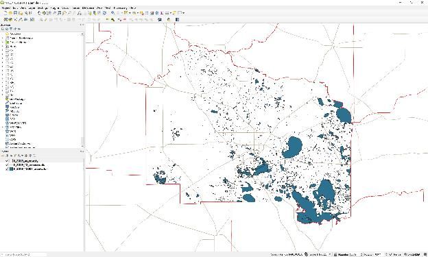
Credit: Young Gu Her and Ziwen Yu, UF/IFAS
Example 2: Counting the Number of People in an Age Group in a County
In this example, a set of US Census survey data will be linked to a TIGER/Line Shapefile to count the populations in the age group of 14 to 17 in Florida. The population census data are tabulated with the dimensions of age and sex attributes aggregated at the county level. The key to this example is to join the tabulated demographic data to the shapefile to map the population data at the county level across the state of Florida.
- To join the two different datasets, the US Census data and the TIGER/Line Shapefile, a common identifier (GEOID) will be used to match each record of the US Census data to objects in the TIGER/Line Shapefile.
- Open up the attribute table of the shapefile.
- To see the county-level population (in the age group of 14 to 17) in this example, select the previously downloaded county boundary layer (“tl_2019_us_county.shp” in “tl_2019_us_county.zip”) of the TIGER/Line Shapefile with the identifier data field, “GEOID,” in the fourth column from the left (Figure 6).
- The GEOID values consist of two digits of “STATEFP” (state FIPS codes) and three digits of “COUNTYFP” (county FIPS codes). The analysis processes strictly follow the Federal Information Processing Series (FIPS) Codes of GEOIDs defined by the US Census Bureau. “FIPS codes for smaller geographic entities are usually unique within larger geographic entities. For example, FIPS state codes are unique within nation and FIPS county codes are unique within state. Since counties nest within states, a full county FIPS code identifies both the state and the nesting county” (US Census 2020c).
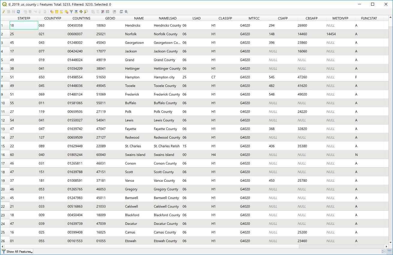
Figure 6. Attribute table of a TIGER/Line Shapefile ("tl_2019_us_county.shp") and its GEOID field.
Credit: Young Gu Her and Ziwen Yu, UF/IFAS - The US Census data (“cc-est2019-agesex-12.csv” and “cc-est2019-alldata-12.csv”) do not have the GEOID values; therefore, the state and county FIPS codes included in the census data need to be combined to create the GEOID values. This data manipulation can be done using common spreadsheet software such as Excel.
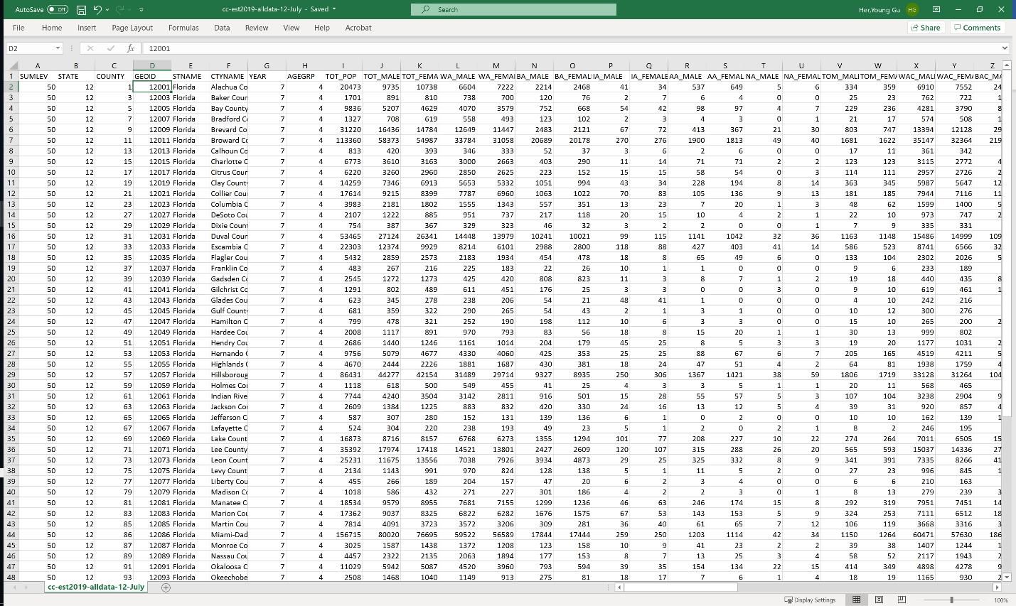
- In the case of the age-sex dataset (“cc-est2019-agesex-12.csv”), for instance, a new field or column (e.g., the field “D”) can be generated by giving the name of “GEOID” to the new field (e.g., in the cell of “D1”) and filling the column with the following formula in Excel: “=TEXT(B2, “000”) & TEXT(C2, “000”)” (Figure 7).
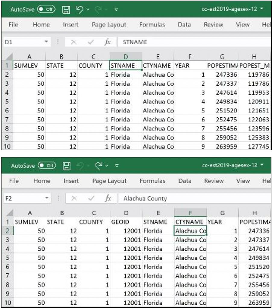
Figure 7. Creating the GEOID field and identifiers in the US Census data ("cc-est2019-agesex-12.csv").
Credit: Young Gu Her and Ziwen Yu, UF/IFAS - The U.S. Census data (“cc-est2019-agesex-12.csv”) have the population data at twelve different time points or periods (from April 1, 2010 to July 1, 2019; https://www2.census.gov/programs-surveys/popest/technical-documentation/file-layouts/2010-2019/cc-est2019-agesex.pdf), which means that each county has twelve rows, but the TIGER/Line Shapefile (“tl_2019_us_county.shp”) has only one polygon per county. Thus, one polygon matches twelve rows, which will prevent them from being joined correctly in GIS software (e.g., QGIS and ArcGIS®).
- Therefore, a specific period (or “time point”) of the population estimates (or data) needs to be selected to solve the one-to-many matching issue.
- In this example, the YEAR key of 7 is chosen, which will lead to investigating the population (or the number of people in the age group of 14 to 17) of Florida’s counties on July 1, 2014. It is worth noting that the “YEAR” column of the US Census data (“cc-est2019-agesex-12.csv”) represents a specific time point for which the corresponding population estimates were made (rather than years or months) (https://www2.census.gov/programs-surveys/popest/technical-documentation/file-layouts/2010-2019/cc-est2019-agesex.pdf).
- Once the period (or “time point”; i.e., July 1, 2014; the YEAR key of 7) of interest is determined, the rows that correspond to the time point of interest will be selected and imported to QGIS for the joining process.
- Use the “join” function in QGIS to join the two datasets that have the common data identifier (GEOID) (Figure 8). To map the population data (or show the spatial variation of the population over counties) using the TIGER/Line Shapefile (“tl_2019_us_county.shp”), the US Census data (“cc-est2019-agesex-12.csv”) will be joined into the shapefile (rather than joining the attribute table of the shapefile into the US Census data).
- Once the joining process is complete, we can map the US Census population data on top of the TIGER/Line Shapefile data (Figure 9).
Credit: Young Gu Her and Ziwen Yu, UF/IFAS
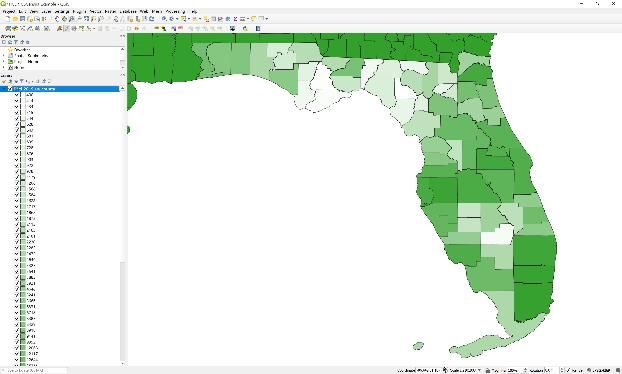
Credit: Young Gu Her and Ziwen Yu, UF/IFAS
Example 3: Mapping Population Compositions by Race and Ethnicity
This example demonstrates how to determine the spatial distributions of the population compositions by race and ethnicity across Florida using the TIGER/Line Shapefile (“tl_2019_us_county.shp”) and the US Census data (“cc-est2019-alldata-12.csv”; https://www2.census.gov/programs-surveys/popest/technical-documentation/file-layouts/2010-2019/cc-est2019-alldata.pdf).
- The US Census data have population estimates (or data) by 18 different age groups. This example will focus on the age group of 15 to 19 (the AGEGRP key of 4) on a particular time point of July 1, 2014 (the YEAR key of 7).
- The US Census data do not have a common identifier data field that matches the GEOID field of the TIGER/Line Shapefile; therefore, an identifier field needs to be created by combining the two digits of the state FIPS and the three digits of the county FIPS code numbers in a spreadsheet (Figure 10).
- Then, the processed population dataset needs to be imported into QGIS and joined to the county shapefile using GEOID.
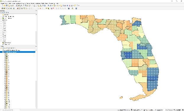
- There are many race, ethnicity, and sex classes. For demonstration, the “Black or African American along female population,” “American Indian and Alaska Native along female population,” and “Two or More Races male population” are selected and mapped in Figures 11 to 13.
Credit: Young Gu Her and Ziwen Yu, UF/IFAS
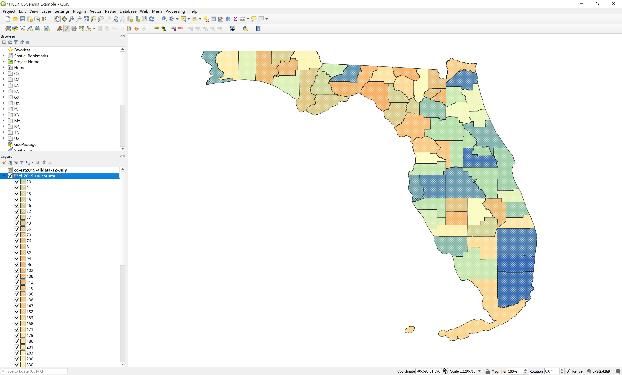
Credit: Young Gu Her and Ziwen Yu, UF/IFAS
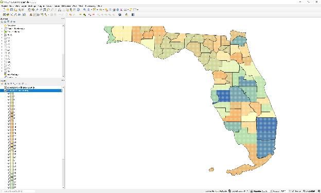
Credit: Young Gu Her and Ziwen Yu, UF/IFAS
Credit: Young Gu Her and Ziwen Yu, UF/IFAS
The TIGER/Line Shapefiles are useful geographic datasets that can help map the spatial variations of variable and attribute data collected for different interests, such as the US Census data. The unique GEOIDs are the key information enabling the integration of the shapefiles and census data at various geographic levels. Users need to pay particular attention to identifying the proper (unique) identifier shared by both shapefiles and survey datasets. The join function of GIS software may only accept one join key, which could be the combination of multiple fields in one of the joining tables.
Summary
The US Census data provide primary information about the American people and the economy on which policy and decision-making rely. The TIGER/Line Shapefiles enable the spatial visualization of the US Census data and help users better understand the demographic features of the areas of interest. This article demonstrates how to map shapefiles, integrate the two datasets, and extract secondary information useful to Extension programs and stakeholders’ decision-making processes. Although the examples provided in this article focus on the county-level analysis of certain demographic features, the methodology can be applied to other combinations of the TIGER/Line Shapefile types (e.g., block and ZIP code area shapefiles and coastal lines; Table 1) and the US Census population datasets. The 2020 Census results, such as the new population counts, were planned to be released in May 2021 (https://www.census.gov/programs-surveys/popest/about/schedule.html). The analysis method presented in this article is expected to help EDIS readers to quickly understand how demographic and economic changes in the United States have occurred over the past decade.
References
DiBiase, D. 2014. TIGER, Topology and Geocoding. Nature of Geographic Information: An Open Geospatial Textbook.
Flenniken, J. M., S. Stuglik, and B. V. Iannone. 2020. “Quantum GIS (QGIS): An Introduction to a Free Alternative to More Costly GIS Platforms.” EDIS 2020 (2). https://doi.org/10.32473/edis-fr428-2020
US Census. 2020a. “Methodology for the United States Population Estimates: Vintage 2019.” Accessed on October 6, 2020. https://www2.census.gov/programs-surveys/popest/technical-documentation/methodology/2010-2019/natstcopr-methv2.pdf
US Census. 2020b. “TIGER/Line Shapefiles.” Accessed on October 6, 2020. https://www.census.gov/geographies/mapping-files/time-series/geo/tiger-line-file.html
US Census. 2020c. “Understanding Geographic Identifiers (GEOIDs).” Accessed on October 6, 2020. https://www.census.gov/programs-surveys/geography/guidance/geo-identifiers.html