Abstract
Energy use in aquaculture is a primary contributor to on-farm operational costs. Pumping water is one of the industry’s most energy-intensive and expensive processes. Most producers inadvertently operate with poorly designed and over-engineered systems. Selecting the correct pump size can significantly reduce energy consumption. The performance characteristics of pumps can be described using pump performance diagrams. These diagrams help to show users how a pump will behave under various conditions by relating characteristics such as flow rate, head, net positive suction head, efficiency, and horsepower. Understanding these characteristics and knowing how to read performance diagrams are crucial to selecting the correct pump size. Pumps must provide the correct combination of flow and pressure to operate properly. After the desired flow rate and construction of a water distribution system is determined, the pressure loss of the water distribution system can be calculated. The total pressure loss of the water distribution system is equal to the minimum amount of pressure a pump must provide to deliver a certain flow rate. By evaluating water distribution systems and determining the minimum requirements of a pump, performance diagrams can be used to help select the correct pump. Pumps and water distribution systems must be matched together to operate efficiently.
Introduction
In the aquaculture industry, energy cost is often the second-largest operational cost next to labor. Although variable in size, most Florida aquaculture facilities consist of outdoor ponds, indoor tanks, or both. Many production systems require water to be continually exchanged and filtered to provide a suitable environment for culturing fish. Opportunities exist to improve aquaculture pumping systems by selecting properly sized pumps. Selecting the correct pump helps to reduce energy consumption, while increasing system life, performance, and reliability. When selecting a pump, characteristics of both the water distribution system and pump must be considered. This publication explains the basic methodology used to size pumps for aquaculture systems; however, these concepts can be applied to a variety of pumping systems. The information discussed is intended to help farmers, researchers, and anyone interested in aquaculture to better understand centrifugal pumps.
Pump Fundamentals
Pumps are machines that create flow by adding energy to fluids. Most pumps in aquaculture are used for moving water to and from production sites, draining ponds, running water filtration devices, and driving circulation. According to a report by Hydraulic Institute, Europump, and the Department of Energy (2004), electric pumps account for nearly 20% of energy used worldwide by electric motors and up to 50% of energy consumption in some industrial facilities. Nearly 90% of all pumps used in the aquaculture industry are centrifugal (Landau 1992). These pumps operate by rotating an encased high-speed impeller. Water is accelerated across the impeller and directed outward as a result of centrifugal force, hence the name (Wheaton 1977). This simple design allows centrifugal pumps to be offered in an array of configurations at relatively low cost. All centrifugal pumps operate on the same premise but can be classified by design and impeller type.
Volute and diffuser pumps are the two most common pump designs used in aquaculture. Volute pumps (Figure 1) are named for their spiral volute-shaped pump case. This simple design is favored for its ability to handle dirty water carrying reasonable amounts of debris. Diffuser pumps (Figure 2) use a concentric pump case with diffuser vanes around the impeller that help to increase efficiency (Wheaton 1977). Both diffuser and volute pump designs are available in many sizes and configurations.

Credit: Wheaton (1977)

Credit: Wheaton (1977)
Centrifugal pumps can use three different kinds of impellers; open, semi-closed, and closed. Open impellers (Figure 3) use vanes attached to a small hub that allow high amounts of debris to pass through the pump unimpeded. Semi-closed (Figure 4) impellers have vanes attached to a single circular base plate and operate more efficiently than open impellers. Semi-closed impellers are preferred for a balance in efficiency and ability to handle moderate amounts of debris. Closed impellers (Figure 5) have vanes between a solid base plate and a face plate, open at its eye. Closed impellers are the most efficient of these three types, but they must be used with debris-free fluid to prevent damage (Wheaton 1977). Semi-closed and closed impellers are most commonly used in aquaculture. Centrifugal pumps are offered in many configurations. Consult a pump professional for recommendations on specific applications.

Credit: Wheaton (1977)

Credit: Wheaton (1977)

Credit: Wheaton 1977
Pump Terminology
How a pump operates can be described by the following terms:
- Flow rate
- Head
- Efficiency
- Net positive suction head (NPSH)
- Cavitation
Flow rate is the volume of fluid a pump can provide per unit of time and is most often expressed in gallons per minute (gpm). For example, a pump may fill a tank at a rate of 50 gallons per minute.
Head is an alternative way of expressing pressure and is used by pump manufacturers to quantify the amount of pressure a pump can provide. Therefore, the term “head” will be used to describe pump pressure for the remainder of this publication. Head is measured in feet, whereas pressure is measured in pounds per square inch (psi). The pressure under 2.3 feet of water is one psi, therefore, one psi is equal to 2.3 feet of water. When dealing with pumping systems, flow rate and head are related. For example, in an aquaculture system, as flow is increased, the pressure in the system must also increase.
Efficiency of a pump is the ratio of work applied hydraulically to the power required to operate the pump. Pump efficiency is represented as a percentage and will depend on how the pump is operated. Neither pumps nor electric motors are 100% efficient. Energy losses, such as those from friction, occur in both the pump and the motor. Pumps operating at their best efficiency point (BEP) will provide the best combination of flow and pressure while consuming the least amount of power.
Net positive suction head (NPSH) is an often overlooked and misunderstood concept of pump selection. NPSH is the pressure at the center of the pump’s suction inlet. Pumps move fluid by creating a vacuum on the suction side of the pump. If the pump does not have adequate suction side flow, the vacuum pressure in the pump can become too great, causing cavitation.
Cavitation is caused when the pressure on the suction side of the pump drops below the vapor pressure of water, resulting in the formation of air bubbles at the impeller. These air bubbles reduce efficiency and cause physical damage to pump internals. In aquaculture, cavitation can lead to gas supersaturation, commonly known as gas bubble disease, and can result in the death of aquatic animals (Parker 1976). Cavitation can be identified by excessive pump noise, unusual vibrations, reduced flow, reduced pressure, and pitted pump internals. Additionally, reduced water flow through the pump can cause overheating and damage to the pump motor and bearings. Common causes of cavitation include blocked suction lines, clogged filters, poor piping design, and unmet NPSH requirements.
Pump Diagrams
Pump performance diagrams are provided by the manufacturer to explain how a pump will operate under different conditions. End users must understand how to read performance diagrams to select the correct pump. These diagrams show plotted curves that relate key performance characteristics such as flow rate, head, NPSH, efficiency, power, pump speed, and impeller size. Although most performance diagrams explain similar information, the content of each diagram will depend on application and manufacturer.
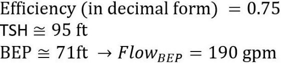
A basic pump performance diagram is shown in Figure 6. This diagram displays a relationship between flow and head for three different pumps. Each of the flow-head curves relates the amount of flow produced at corresponding head values for that specific pump. A pump will always provide a combination of flow and head somewhere on the curve. Pump power, speed, and impeller size will be identifiable through the manufacturer’s pump literature if not provided with the diagram. When efficiency curves are not shown on the diagram, the best efficiency point can be estimated at 75% or 85% of the pump’s total shut-off head. Total shut-off head (TSH) is where the flow-head curve intersects the left-hand vertical axis, and it is the pump’s maximum head (pressure) capability. It is recommended by pump professionals to use 75% of TSH for 3600 rpm pumps and 85% of TSH for 1800 rpm pumps. For example, using Figure 6 and the equation below, it can be estimated that Pump A fitted with a 3600-rpm motor will operate most efficiently when providing approximately 71 ft of head and a flow rate of 190 gpm.
BEP(ft) = Efficiency x TSH(ft)
where:

Credit: Courtesy of Pentair
A more comprehensive pump performance diagram for a centrifugal pump is shown in Figure 7. The diagram includes curves that relate flow rate, head, efficiency, power, and impeller size. The flow-head curves relate the amount of flow produced at corresponding head values. Efficiency curves shown in green indicate the efficiency of the pump across the operating range. The BEP for the pump fitted with a 6.61-inch impeller is 75.8%; here, the pump will provide 147 gpm at 36 ft of head. Power requirements, indicated by the dashed lines, specify the power necessary to operate the pump under various conditions. Operating the pump at any point on the head-flow curve between the dashed 1.5 hp and 2 hp power curves would require a 2 hp motor. The area inside the shaded region between the two flow-head curves indicates the preferred operating range of the pump. Manufacturers sometimes set preferred operating ranges to show users where the pump can safely operate. Additionally, the bottom diagram is shown to indicate the required NPSH of the pump at different operating points. If the performance diagram does not supply an NPSH curve, the pump manufacturer should provide a minimum value. Further discussion of NPSH is included in the “Pump Selection” section of this publication.

Credit: Courtesy of MDM Inc.
Pump Selection
Choosing a pump for any application requires the user to evaluate the water distribution system and determine the following:
- Flow rate
- Head requirement
- NPSH available
The design of a water distribution system will affect how a pump performs. Water distribution systems are networks of pipes that control the movement of water from one place to another. Most aquaculture producers use similarly designed systems, predominantly constructed of PVC pipe. These systems consist of pipes, filters, valves, and other fittings such as tees, elbows, couplings, and discharge nozzles. As the demand for flow in a system increases, the amount of pressure produced by a pump must also increase to overcome the resistance of moving water through pipes, fittings, and other components. The magnitude of these resistances is largely a function of water speed in the pipe, pipe diameter, pipe length, and the vertical distance water must be pumped.
The desired flow will depend on the specific needs of the user, often contingent on production size, system type, and species of fish cultured. Flow rate can be determined by totaling the desired flow rates of all the discharge points. Due to the redundancy in most aquaculture systems, the total flow rate can be calculated by determining the flow rate at one discharge point and multiplying it by the total number of discharge points in the system. The flow rate of a discharge point can be measured using the simple bucket and stopwatch method. Place a container of known volume under a discharge point and record the amount of time it takes to fill the container. For example, if a one-gallon bucket takes 30 seconds to fill up, the flow rate at that discharge point must be two gpm. If using a five-gallon bucket to perform this test, be aware most buckets advertised as five gallons are not exact. Actual volume is dependent on manufacturer.
The head required by a pump can only be determined after the desired flow rate is defined. This is because the amount of head a pump must produce to overcome the resistance of pumping water is dependent on flow rate. As the amount of flow in a system increases, the amount of head required to deliver that flow must also increase. The head requirement can be determined by calculating the total head loss in the system using the equation below. The total head loss in a water distribution system is the minimum pressure a pump must provide to deliver a desired flow rate. Total head loss is the sum of the vertical distance water must be pumped () and the friction head loss (). Friction head loss is the loss of pressure caused when water flowing through pipes and fittings is slowed down by frictional resistance. Moving water through the water distribution system creates additional resistance for the pump. The calculation of frictional losses is beyond the scope of this document, but it can be approximated by using this online friction head loss calculator. If using a different method to determine frictional losses, be sure to use an approach that accounts for multiple outlets along a single pipe.
Total Head Loss – Hz + HLf
where:
NPSH of a pumping system can be separated and explained by two terms, NPSHrequired and NPSHavailable. The is the minimum pressure required at the pump’s suction inlet to avoid cavitation. NPSHrequired is a predetermined value and is supplied by the pump manufacturer. NPSHavailable is the amount of pressure in the water distribution system available at the pump suction inlet. It is important to understand that is dependent on the design of the suction side piping, not the pump. The NPSHavailable must be equal to or greater than the NPSHrequired. Insufficient will lead to excessive vacuum pressure at the pump’s suction inlet, causing cavitation and other performance issues. For aquaculture systems with vented or open-top tanks pumping water at or near 80⁰F, use the formula below to determine NPSHavailable. The friction loss on the suction side of the pump can be estimated using the calculator in this link. Fittings can add to frictional losses, so be sure to follow the instructions in the calculator and account for them.
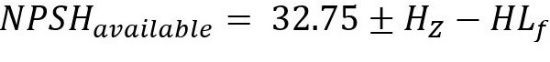
where:
After the desired flow rate, head requirement, and the are determined, a pump can be selected using pump performance diagrams. The selected pump should be the one that provides the desired flow and head most efficiently. It is not likely that an off-the-shelf centrifugal pump will satisfy the exact head and flow requirements of the end user. Therefore, it would be wise to select a slightly oversized pump that can efficiently handle additional flow rate in case of future expansions. However, pumps should not operate long term at more than 10% less than the BEP. Operating a pump at a point on the head-flow curve to the left of the BEP leads to a reduced flow that can cause bearing failure, overheating, and cavitation. Operating a pump too far to the right of the BEP changes the NPSH requirements, which can also lead to cavitation. On occasion, frequent changes in flow are required. This can be accommodated by using multiple pumps or variable speed drives. If a large reduction in flow is desired, using bypasses can recirculate extra water back into sumps and keep pumps operating efficiently.
Design Considerations
Poorly designed water distribution systems can restrict function and efficiency. Plumbing nearest the pump should be designed to limit irregularities in flow. Elbows, tees, large reducers, and check valves near the pump inlet can cause turbulent flow in the pipe, leading to cavitation and harsh vibration. Additionally, an excessive amount of pipes, fittings, and valves add to frictional head losses. For example, adding a two-inch schedule 40 PVC elbow to a pipe is equivalent to adding an additional 5.17 feet of straight pipe. Limiting water velocity to 5 feet per second (ft/s) or less also helps minimize pressure loss in the system due to friction. The following equation can be used to calculate water velocity in a pipe. The inside pipe diameter should always be used when calculating water velocity. Table 1 lists inside diameters for schedule 40 PVC pipe and water velocity for some predetermined flows. Furthermore, using pipe diameter large enough to prevent water velocities from exceeding 5 ft/s will reduce the risk of damage to pipes and pumps caused by water hammer (Clark 1988).
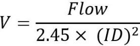
where:
V = Water velocity (ft/s)
Flow = total flow in the pipe section (gpm)
ID = Inside pipe diameter (in)
Piping at the pump’s suction inlet should have a minimum length of five times the pump’s inlet diameter. For example, a pump with a two-inch inlet should have a minimum of 10 inches of straight pipe before the pump. Reducers and elbows should be positioned away from the pump’s inlet and discharge flanges. Eccentric reducers should be used instead of traditional concentric reducers on suction lines. Install reducers so the flat side is on the top when water is coming from below or straight to the pump, and on the bottom when water is coming from above the pump. The use of traditional concentric reducers at the suction inlet can lead to premature wear and reduced efficiency.
Pumps are available in multiple electrical configurations, so attention to surrounding electrical infrastructure is important. Pumps under five horsepower can be fitted with single- or three-phase electric motors and are often available in either configuration. Single-phase motors are offered in both 120- and 220-volt options and can often be configured for either voltage. Most pumps at five horsepower or greater are fitted with three-phase electric motors. Three-phase is available in several high- and low-voltage configurations depending on the service provider’s infrastructure. Three-phase pumps operate more efficiently and are often less expensive. However, installing a new three-phase service can be costly; if it is not required, the cost benefit should be considered. Even though three-phase systems transmit more power, they often use smaller wire and simpler motor designs. When facilities use many large pumps, this can help offset the cost of installing a new three-phase service. Three-phase power has a high initial cost but is usually the least expensive option in the long term.
Conclusion
It is important for end users to understand how a pump will operate under specific conditions to ensure the pump will meet their requirements and operate efficiently. When selecting a pump for an aquaculture system, the desired flow rate, head requirement, and the must first be determined by evaluating the water distribution system. After establishing the necessary requirements, pumps can be selected using performance diagrams. These diagrams make it possible to predict the behavior of a pump under specific conditions. The efficient operation of pumps and pumping equipment is dependent on balanced interactions among many system components. By selecting the proper pump and avoiding a one-size-fits-all mentality, on-farm energy consumption and operational costs can be greatly reduced. If necessary, end users should consult with pump manufacturers and professionals during selection and installation.
References
Blankston, D. 2013. “Piping Systems.” Southern Regional Aquaculture Center 373.
Clark, G., and D. Haman. 1988. “Water Hammer in Irrigation Systems.” 828. Gainesville: University of Florida Institute of Food and Agricultural Sciences.
Haman, D. 1994. "Pumps for Florida Irrigation and Drainage Systems." 832. Gainesville: University of Florida Institute of Food and Agricultural Sciences.
Hydraulic Institute, Europump, and US Department of Energy. 2004. "Variable Speed Pumping. A Guide to Successful Applications, Executive Summary."
Landau, M. 1992. Introduction to Aquaculture. John Wiley & Sons Inc.
Parker, N., K. Strawn, and T. Kaehler. 1976. "Hydrological Parameters and Gas Bubble Disease in a Mariculture Pond and Flow-Through Aquaria Receiving Heated Effluent." Journal of the Southeastern Association of Fish and Wildlife Agencies:179–191.
Washington State University Extension. n.d. "Pressure Loss with Outlets." Irrigation in the Pacific Northwest. http://irrigation.wsu.edu/Content/Calculators/General/Pressure-Loss-With-Outlets.php
Wheaton, F. 1977. Aquaculture Engineering. 356–413. Robert E. Krieger Publishing Company.
Table 1. Water velocities in schedule 40 PVC pipe. Highlighted values are beyond the normally preferred maximum velocity.