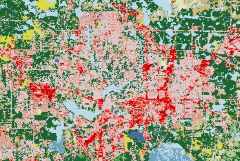
FRAGSTATS: A Free Tool for Quantifying and Evaluating Spatial Patterns
Abstract
Human activities such as urbanization and agriculture have triggered rapid land cover change, resulting in the loss of natural ecosystems and the ecosystem services and biodiversity that these ecosystems provide. Therefore, understanding land cover change and its environmental impacts is a key issue in future land-use planning. The first step for planning is the ability to quantify patterns of land cover objectively. However, quantifying these patterns can be difficult without the proper resources. In this document, we introduce one such resource, a free software called FRAGSTATS that is capable of quantifying spatial patterns in land cover. The ability to quantify these spatial patterns and their changes over time can guide land-use planning. We illustrate the utility of FRAGSTATS by walking the readers through the steps of analyzing changes in land cover patterns for urban and upland forested areas in Alachua County, Florida, from between 2001 to 2011. The reader will learn how to create input data, run FRAGSTATS, and interpret outputs. Although we introduce some basic concepts of landscape ecology and GIS, this document is intended for those individuals already having experience using GIS packages such as ArcGIS and QGIS for basic procedures (e.g., mapping, data visualization).
Introduction
What is land-use change?
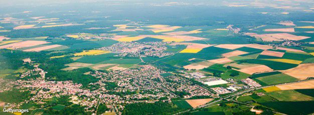
Looking at the surface of Earth from an airplane, one can see a mosaic of forests, grasslands, lakes, cities, farmlands, and more (Figure 1). Each of these land cover types exhibits different ecosystem functions and properties, and collectively all the types form what ecologists refer to as a landscape.
Credit: USDA
Currently, landscapes are changing dramatically via the expansion of both urban and agricultural land cover types. These changes, which are referred to as land-use change, have inevitable environmental impacts. For instance, forests and wetlands, which used to be dominant land cover types in Florida, continue to be converted into agricultural and urban lands (Kautz et al. 2007). With the conversion of forests and wetlands to other land cover types comes the loss of the many ecosystem services and functions that these ecosystems provide. A description of these ecosystem services can be found in various chapters of the United Nation's Millennium Ecosystem Assessment (MEA 2005a; MEA 2005b).
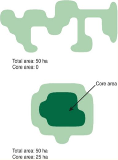
Land-use change not only causes losses in total area of given natural and seminatural land cover types, but also changes in the spatial arrangement of these land cover types, the loss of important core habitat provided by these land cover types, and an increase in edge habitat (Shao et al. 2018; Murcia 1995). The distinction between core and edge habitat is important because each exhibit different characteristics. Habitat edges experience greater effects from nearby land cover types and thus greater levels of stressors in urban areas, including increased pollution and invasive plants. In contrast, core habitats, i.e., the areas at the center of habitat areas, exhibit characteristics typical of less-disturbed ecosystems. They are often critical for conservation efforts and for maintaining the ecosystem services that these habitats provide. Some species do quite well in edge habitats because they are able to gather resources from multiple types of ecosystems. For these reasons, we need to determine not only how land-use change affects the total area of different land cover types, but also the spatial arrangement, and amounts of core vs. edge habitats that these land cover types provide. Being able to quantify these changes is of critical importance for future land-use planning in order to ensure that our future choices regarding how we alter landscapes are more environmentally responsible.
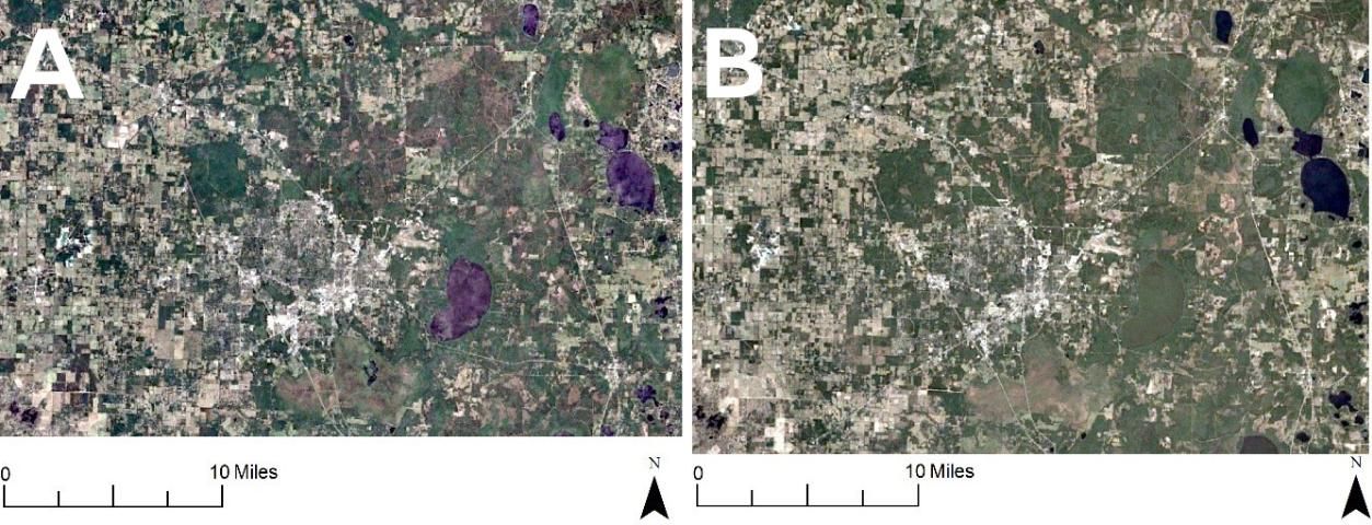
So how can we do this? We could simply compare satellite images taken at different times, but trying to perceive changes in land cover types simply by looking, let alone quantifying those complicated patterns precisely, would be difficult if not impossible. Satellite images of Alachua County, Florida, from 1984 and 2016 demonstrate this point (Figure 2). While it is relatively easy to detect some changes in land cover types, measuring amounts and differences in spatial patterns visually or by hand would be challenging.
Credit: Google Earth
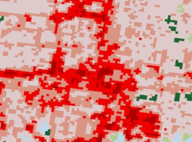
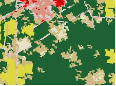
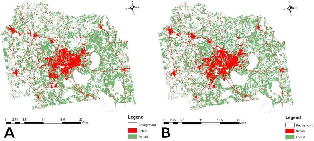
One way that land-use change can be quantified is by dividing each map into cells and then assigning each cell a land cover type (e.g., urban, forest, grassland, wetland, agricultural land). The size of each cell (i.e., "resolution") for such data varies depending on different data sources. For data on larger spatial scales, cell resolution will usually be 1 km2, 300 m2, or 30 m2. For more information about land cover types and standard classification procedures, please check https://archive.usgs.gov/archive/sites/landcover.usgs.gov/classes.php.html. This post-processed land cover map is referred to as a raster map. To give a better overview of what a raster map is, we provide two maps of the urban and upland forest land cover of Alachua County, Florida, in 2001 and in 2011 (Figure 3). Urban cells are colored red, and upland forest cells are colored green. White cells are various other land cover types. Even this simplified depiction of changes in upland forest and urban cover, while easier to visualize than initial land cover images (e.g., Figure 2), would be challenging to quantify by hand or visually.
Credit: Google Earth
To assist in quantification, designers created FRAGSTATS, a free software that can quantify spatial patterns of land cover from rasterized maps. Using FRAGSTATS on two photos taken at two locations or at two different periods (e.g., Figure 3) allows for quantification of differences and changes in land cover over time. Such information is critical for making decisions about land development and for the conservation of habitat and habitat core areas provided by different land cover types.
Introduction to FRAGSTATS: An Example of Land-Use Change in Alachua County, Florida.
The FRAGSTATS team periodically updates the software and provides technical support. For this case study, you will need to download FRAGSTATS from http://www.umass.edu/landeco/research/fragstats/downloads/fragstats_downloads.html#FRAGSTATS. The version described in this fact sheet is 4.2. In addition, we highly recommend you download the help document for FRAGSTATS, which provides much more detail about FRAGSTATS than is practical in a short fact sheet: https://www.umass.edu/landeco/research/fragstats/documents/fragstats.help.4.2.pdf.
Below we present a case study to better demonstrate how FRAGSTATS works. In this case, we focus on the land cover change in Alachua County, Florida, from 2001 to 2011, a period over which urbanization has changed the total area and spatial arrangement of natural areas. We illustrate the utility of FRAGSTATS by using it to quantify spatial changes in urban and upland forest land cover types between 2001 and 2011.
Before we jump into our introduction of FRAGSTATS, one step cannot be missed. FRAGSTATS does not support the raster data visualized in Figure 3. It instead works off integer grids in which each grid cell is directly assigned an integer value corresponding to the class of land cover type dominating that cell. Therefore, we need to convert the maps shown in Figure 3 to integer grids. Typically, FRAGSTATS prefers integer grid files in the GeoTIFF and/or ASCII format. This conversion can be done using ArcGIS or other GIS software. Figure 4 shows an example of a GeoTIFF file in which the gray cells represent urban areas, white cells represent upland forests, and black cells represent other land cover types merged into one class of land cover type.
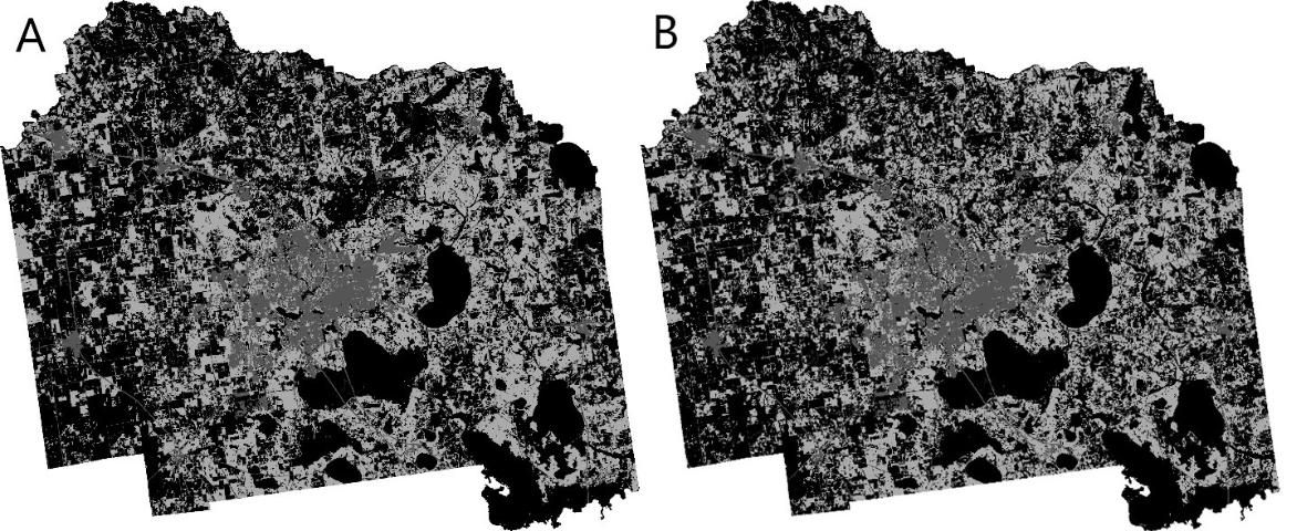
We provide the two GeoTIFF files required for this exercise via the Institutional Repository at the University of Florida at https://ufdc.ufl.edu/IR00011008/00001?search=iannone. To work through this example, download the entire folder to your desktop. The first GeoTIFF file named "UrbanForestsCover2001.tif" shows the land cover for Alachua County, Florida, in 2001. The other GeoTIFF file entitled "UrbanForestsCover2011.tif" shows the same, but for 2011. This folder also contains a text file named "ClassDescriptor" needed to run our example, as explained below, and a Word document entitled "How a tiff file is created" describing how to convert raster files to GeoTIFF files using GIS software. Again, for the purpose of this document, we have completed this step for you.
Working with Example Files
Open FRAGSTATS, then click on "File" in the upper left corner and select "New" from the dropdown menu. Afterward, you will see the console shown in Figure 5. Here we provide a brief introduction about different sections in this console.
Section 1 in Figure 5 is the menu bar, where we can create, open, save, or run analyses on an integer grid file map (e.g., Figure 4).
Section 2 of Figure 5 has two tabs in the upper left. The tab entitled Input Layer is where we input or remove data, i.e., GeoTIFF/ASCII files generated from GIS raster data. The tab entitled Analysis Parameters is where we specify extra parameters or sampling methods (Figure 6).
Section 3 of Figure 5 is where we specify what FRAGSTATS refers to as the common tables; important parameters that are necessary for running FRAGSTATS are specified here. More information about the common table area is provided below.
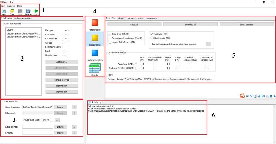

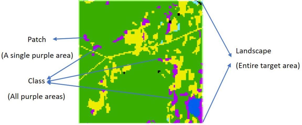
Section 4 is for selecting the scales at which metrics will be calculated: Patch, Class, and/or Landscape, as depicted in Figure 7. A patch is an area of a homogenous land cover type that differs from its surroundings (Forman 1995). A class is a group of patches that share the same land cover type. Landscape usually represents the area of interest—for our example, Alachua County, Florida. The scale on which to estimate metrics depends on the research objectives.
After selecting the scale at which metrics will be calculated, we need to choose specific metrics that we want to calculate. This selection is done in Section 5 of Figure 5. Note that the specific choices of metrics vary depending on the selected scale (i.e., patch, class, or landscape). FRAGSTATS divides metrics into 5 groups, including area and edge, shape, core area, contrast, and aggregation. To select these different metric groups, click on the tabs shown at the top of Section 5 in Figure 5. The spatial aspects being quantified by each of these metric classes are defined in Table 1.
Finally, Section 6 of Figure 5 is where the program shows its activity log, including errors or processing information. The purpose of these sections will become clearer as you work through this example.
The document called fragstats.help.4.2 is a user guide that provides detailed explanations about the background of FRAGSTATS, how FRAGSTATS works, and the explanation of the different metrics and parameters. In addition, you can click "help" on the menu bar, i.e., Section 1 of Figure 5, to learn more.
Now that we have explained the FRAGSTATS console as well as metric scales and types, we will show how FRAGSTATS works by quantifying changes between 2001 and 2011 in spatial aspects of urban and upland forest cover in Alachua County, Florida.
First, input the GeoTIFF files of Alachua County land cover in 2001 and 2011. Click the button "Add layer" shown in Section 2 of Figure 5, and a dialog box will pop up (Figure 8). Next, select the data type you will use by clicking on the corresponding line in the left pane. In this example, it would be GDAL Geotiff grid (.tif). Next, click on "..." to the right of the upper right-hand box, navigate to the folder on your desktop, select the file entitled "UrbanForestCover2001.tif," and click OK. Once the first file has been uploaded, repeat these same steps to upload the file entitled "UrbanForestCover2011.tif."
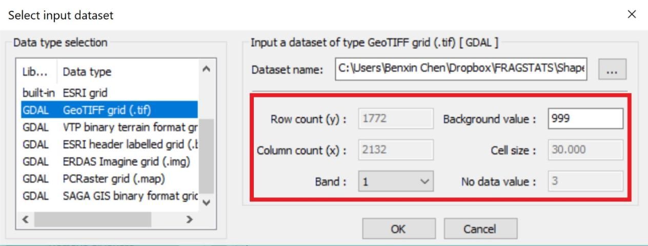
While uploading "UrbanForestCover2011.tif," look to the right pane outlined in red in Figure 8. Row count and column count show the number of cells in the rows and columns, respectively, of the uploaded GeoTIFF file of Alachua County, Florida. Cell size defines the size of each grid in the GeoTIFF file. In our example, each grid is 30 x 30m. Some images may have multiple bands (i.e., layers). You may choose which band to import into the band box. There is only one band in our example. Some GeoTIFF files may contain cells having no data or that are not of interest for the objectives of an analysis (e.g., white cells in Figure 3 and black cells in Figure 4). The value for these cells is assigned in the "no data box". Background value is the value shown for background cells, which are cells beyond the area we are analyzing, i.e., Alachua County, Florida. The program will not calculate values using information from this area of the GeoTIFF image.
After uploading the GeoTIFF files, click on the "Save as" icon shown in Section 1 of Figure 5. Projects in FRAGSTATS are called "models." Name the current model "Alachua," and save it to the folder on your desktop containing the GeoTIFF files.
The next step is to specify the common tables: class descriptors, edge depth, edge contrast, and similarity (Section 3 of Figure 5). For this example, we only need to specify "class descriptor" and "edge depth." The class descriptor is a text file that contains information on the integers used to specify different land cover types and other information, as shown in Figure 9. We have provided class descriptor in the text file entitled "ClassDescriptor.txt." (Note that you can create your own class descriptor using Notepad.) Upload this text file by clicking on the browse button shown in Section 3 of Figure 5, making sure to specify that you want to view "all files (*.*)." As shown in Figure 9, we set "1" to represent "urban" and "2" to represent "upland forest," and "0" as "background." Essentially, what the user needs to know is described in four values: ID, Name, Enabled, IsBackground. For instance, the first row explains that 0 is named "background," and background cells are not to be used ("false") to calculate metrics.
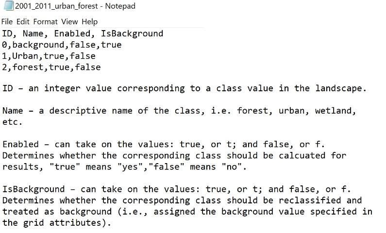
Next, we will specify the edge depth used to estimate metrics on core areas of patches (Table 1). Edge depth defines how wide edges of patches are. In this example, click "use fixed depth" box and set the value to 100, i.e., 100m, by clicking on the navigate button ("...") shown in Section 3 of Figure 5. We selected 100m as our edge depth because effects of edges are detected even at this large of a distance from forest edges (Laurance et al. 2002). For this example, we will not specify parameters for the edge contrast or similarity boxes. To learn more about the functionality of these boxes, please see "USER GUDIELINES?Running via the Graphical User Interface?Step 4. Specifying Common Tables [optional]" section (Pages 54–60) in the "FRAGSTATS help 4.2" document.
In our example, the main interest is in quantifying how upland forest and urban areas (i.e., two land cover types) have changed in area and spatial pattern over time. Therefore, we are only interested in calculating metrics at the class level. Click on the "Analysis parameter" tab shown in Section 2 of Figure 5 and click the box before "Class metrics" under "Sampling strategy" and "No Sampling" in Figure 6.
Next, highlight "Class metrics" in Section 4 of Figure 5 and then choose the target metrics in Section 5 of Figure 5. All of the metrics we will estimate, and the tab under which they are found, are listed in Table 2. Simply check the boxes for each metric in their respective tab, and note when selecting Total Edge (TE) that you will need to specify what "edge" is by clicking the "..." after "Count all background/boundary interface as edge," and selecting "Count all as edge" in the box that pops up. Please refer to "FRAGSTATS METRICS" section of the "FRAGSTATS.help 4.2" document (Pages 76–170) for definitions of these and the many other metrics that FRAGSTATS can calculate.
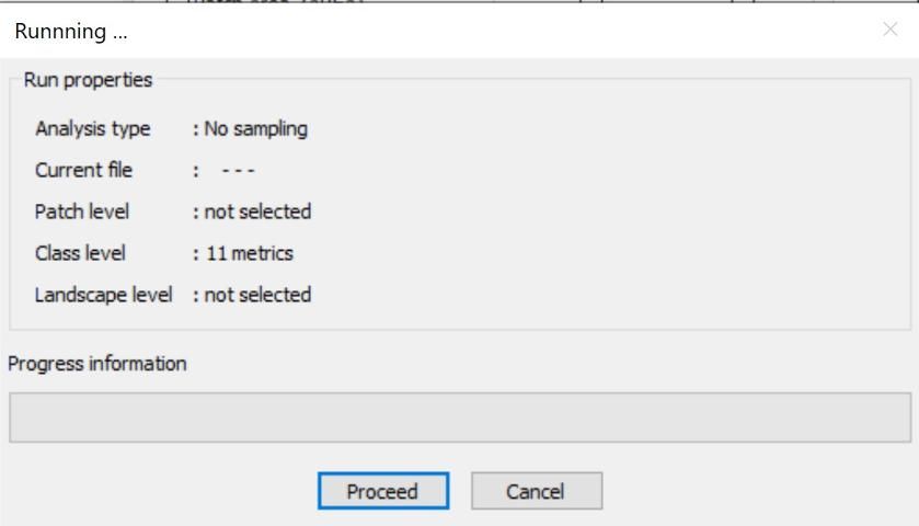
Finally, click "Run" in Section 1 of Figure 5. A progress window, as shown in Figure 10, will pop up: click "Proceed." To see results, click on the "Results" tab in Section 4 of Figure 5, making sure that the "Class" tab is selected (Figure 11). Results will be shown in the results window to the right.
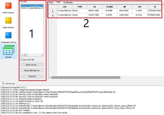
We can check results for the different input GeoTIFF files by highlighting different files listed in the run list (Section 1 of Figure 11). Now look at the table in Section 2 of Figure 11. The first row contains values for spatial metrics calculated for upland forests, while the second row shows the same metrics calculated for urban areas. Both rows are reporting calculations for the GeoTiff file highlighted in Section 1 of Figure 11. We define each metric below when we describe how to interpret model outputs.
Spatial Inferences Revealed
The numerical output generated by FRAGSTATS for the GeoTIFF files depicting land cover change in Alachua County, Florida, provides an understanding of not only how total area of upland forest and urban land cover has changed, but also how the spatial arrangement of land cover types has changed.
This understanding is gained by the many spatial metrics that FRAGSTATS calculates. We calculated three types of metrics, including area–edge metrics (Table 3), core area metrics (Table 4), and aggregation metrics (Table 5). Each specific metric is defined in its respective table.
Through calculating area and edge metrics (Table 3), we found upland forests are not only shrinking in total area, but upland forest patches are also shrinking and becoming more fragmented. For instance, declines in CA and %PLAND show that the total upland forests area in Alachua County declined by an amount that might not seem concerning (0.5%). However, we found that the remaining forest patches decreased in size (AREA_MN) by an average of close to 1 ha. In addition, the 1,145,040 m increase in TE shows that there is now more forest edge in 2011 as compared to 2001, a sign of fragmentation.
These metrics reveal that urban areas, in contrast with upland forests, are not only becoming larger but also more consolidated. Total urban area increased by 0.6% between 2001 and 2011, as revealed by increases in %PLAND. Unlike forest patch size, urban patch size (AREA_MN) on average increased by 1.6 ha while urban edge (TE) increased by 28,000 m (less than the increase exhibited by upland forests). An increase in urban patch size in conjunction with smaller increases in edge suggests that increases in urban areas occurred largely via the growth of existing urban areas.
The result of core area metrics calculation (Table 4) reveals a great loss of upland forest core area. This decline in core area would go undetected in an interpretation that considered only the total area. To be specific, TCA and %CPLAND of upland forests have declined by about 18.9%. In addition, the size of the mean core area of upland forest has decreased by 22.3% (From 3.6 ha to 2.8 ha). This result confirms that though the loss of total upland forest area seems minor, in fact the upland forests are experiencing considerable fragmentation.
In contrast to upland forest areas, the urban areas in Alachua County are experiencing increases in their core. For instance, the increases in TCA and %CPLAND shown in Table 4 reveals a 14.2% increase in urban core areas. In addition, the mean size of urban core areas (CORE_MN) has increased by 0.7 ha, from 4.4 ha to 5.1 ha. The rate of increase of urban core areas in Alachua County is greater than the rate of increase for the total urban area (Table 3), suggesting that sprawl from existing urban areas is contributing to urban expansion more than the emergence of isolated urban areas.
Metrics pertaining to aggregation (Table 5) reveal that overall upland forest area did not only shrink between 2001 and 2011, but it also became more fragmented. For example, the number of patches of upland forests increased from 5,618 to 5,865. Furthermore, the splitting index, which increases with more fragmented patches, rose from 579.1 to 886.1 from 2001 to 2010. These changes in value suggest an increase in the number of upland forest patches due to upland forests becoming more fragmented.
On the other hand, these same metrics reveal that urban patches became more aggregated between 2001 and 2011. This is because the number of urban patches decreased, as does the splitting index, suggesting that urban patches converged somewhat during this period.
One final note, while this case study shows the utility of FRAGSTATS for quantifying spatial patterns, outputs are only as good as the quality of the data used in an analysis. This case study relied on the high-quality National Land Cover Data set from the US Geological Survey. Other datasets may not be of this quality. In addition, data quality may change over time. These changes, along with data spatial resolution and changes in protocols for land cover classification can all affect FRAGSTAT outputs. Therefore, data products should be carefully selected to ensure that they have the characteristics and quality needed to meet the objectives of a given analysis.
Conclusion
While we can see patterns of change in land cover types by looking at maps taken at different times, it is difficult to quantify that change. Nevertheless, such information is needed for making management and planning decisions. FRAGSTATS is a free tool that provides such information. We illustrated its utility for spatial patterns of upland forests and urban areas of Alachua County, Florida. FRAGSTATS revealed that although the decline in the total upland forest area between 2001 and 2011 was low, upland forests have experienced considerable fragmentation and loss of core forest habitat. Aggregation metrics also support this conclusion. For the urban areas, FRAGSTATS reveals not only an increase in the total urban area, but that this area has converged between 2001 and 2011. The fact that fragmentation of upland forests has increased, core upland forest habitat has been lost, and urban areas have converged would have gone undetected had we not relied on FRAGSTATS to quantify spatial patterns in addition to total areas. Precise metrics of these spatial changes are required for long-term decision making regarding regional planning and the conservation of important native, core habitats. FRAGSTATS provides such information, and, given that it is free, should be of great utility as an extension to GIS analyses of land-use change, helping to guide land-use planning.
Additional Resources for Learning FRAGSTATS
Here we provide links to other useful websites in case you are interested in learning more about FRGASTATS.
The current version of FRAGSTATS is 4.2. Information on this version can be found here: http://www.umass.edu/landeco/research/fragstats/fragstats.html
FRAGSTATS and FRAGSTATS updates can be downloaded here: http://www.umass.edu/landeco/research/fragstats/downloads/fragstats_downloads.html
Documentation (e.g., FRAGSTATS help, FRAGSTATS background, etc.) can be found here: http://www.umass.edu/landeco/research/fragstats/documents/fragstats_documents.html
Video and PowerPoint presentations from FRAGSTATS workshops can be found here: http://www.umass.edu/landeco/research/fragstats/workshops/fragstats_workshops.html
Literature Cited
Forman, R. T. T. 1995. "Some general principles of landscape and regional ecology." Landscape Ecology 10:133–142. https://link.springer.com/article/10.1007/BF00133027
Kautz, R., B. Stys., and R. Kawula. 2007. "Florida vegetation 2003 and land use change between 1985–1989 and 2003." Florida Scientist 70:12–23. http://www.orange.wateratlas.usf.edu/upload/documents/Fl_vegetation_2003_and_land_use.pdf
Laurance, W. F., T. E. Lovejoy, H. L. Vasconcelos, E. M. Bruna, R. K. Didham, P. C. Stouffer, C. Gascon, R. O. Bierregaard, S. G. Laurance, and E. Sampaio. 2002. "Ecosystem decay of Amazonian forest fragments: a 22-year investigation." Conservation Biology 16:605–618. https://conbio.onlinelibrary.wiley.com/doi/full/10.1046/j.1523-1739.2002.01025.x
Ecosystems and Human Well Being: Current State & Trends, Volume 1. "Millennium Ecosystem Assessment." 2005a. Washington, DC: Island Press 585–621. https://www.millenniumassessment.org/documents/document.766.aspx.pdf
Ecosystems and Human Well Being: Current State & Trends, Volume 1."Wetlands and Water." 2005b. Washington, DC: Island Press 30–38. https://www.millenniumassessment.org/documents/document.358.aspx.pdf
Murcia, C. 1995. "Edge effects in fragmented forests: implications for conservation." Trends in Ecology & Evolution 10: 58–62. https://www.sciencedirect.com/science/article/pii/S0169534700889776
Shao, G., B. V. Iannone III,, and S. Fei. 2018. "Enhanced forest interior estimations utilizing LIDAR-assisted 3D forest cover map." Ecological Indicators 93:1236–1243. https://www.sciencedirect.com/science/article/pii/S1470160X18304771


