Introduction
Precision agriculture is an expanding field that helps farm managers and agriculture consultants to monitor crops and make intelligent decisions that ultimately help crop growers. Field data can be obtained in the form of digital images from cameras mounted on drones, tractors, and other platforms. One of the main challenges, however, is to extract useful information from these image data. This process typically requires specialized skills and software.
The purpose of this publication is to present a step-by-step guide to image analysis for researchers who use ArcGIS software. Specifically, this guide will allow anyone with basic geographic information system analysis skills to implement the Mask Region Convolutional Neural Networks (Mask RCNN) model, one of the most widely used models for object detection, to delineate strawberry canopies. This is accomplished using the ArcGIS Pro version 2.5 Image Analyst Extension in a simple workflow. The software interface of each step in the workflow is explained with input examples. The results of this demonstration as well as the data used in the training process are available as supplemental material as indicated in the “Data Availability” section at the end of this publication.
Background
Remote sensing image acquisition is becoming increasingly common across agricultural applications. Other UF/IFAS publications illustrating how to acquire drone images (Kakarla, de Morais Nunes, and Ampatzidis 2019) and how to perform post-flight analysis for agricultural applications were recently published (Kakarla and Ampatzidis 2019). This publication provides simple techniques to apply state-of-the-art deep learning methods to delineate strawberry canopies, which is a step in extracting individual plant information used in many applications such as yield prediction and phenotyping. We will demonstrate how to use the ESRI ArcGIS Pro software Image Analyst Extension (ESRI 2019), one of the most widely used GIS software platforms in the world. The University of Florida has a campuswide license that is used by most government agencies in Florida. The dataset used in this article is the same dataset used in Guan et al. (2020) and Abd-Elrahman et al. (2020). The results obtained using the ArcGIS Pro software are compared to the ones achieved by Abd-Elrahman et al. (2020). ArcGIS Pro v 2.5 software was used to prepare this dataset and implement the delineation.
Recently, several deep convolutional neural network (DCNN) algorithms have gained momentum in different image analysis applications, mainly due to their superior object detection, semantic segmentation (classification) performance, and ability to self-extract image features. In the meantime, one of the main factors hindering DCNN implementation on a wider scale is the need for technical computer programming and operating system skills that are not widely held by staff working in the agricultural application field. The objective of this publication is to facilitate the use of deep learning image analysis by introducing a simplified, step-by-step process that implements a widely used software package. One of the most successful DCNN applications is object detection and instance segmentation (Zhao, Zheng, Xu, and Xi 2019). In this article, Mask RCNN architecture (Ammirato and Berg 2019; He, Gkioxari, Dollar, and Girshick 2017) will be deployed. The mathematical and technical aspects of the RCNN implementation are outside the scope of this publication, and interested users can learn more about DCNN in general and RCNN specifically by referring to many available resources listed in, for example, Zhao, Zheng, Xu, and Xi (2019) and Ding, Zhang, Jia, and Chang (2019).
Implementation Steps
- Dataset Preparation
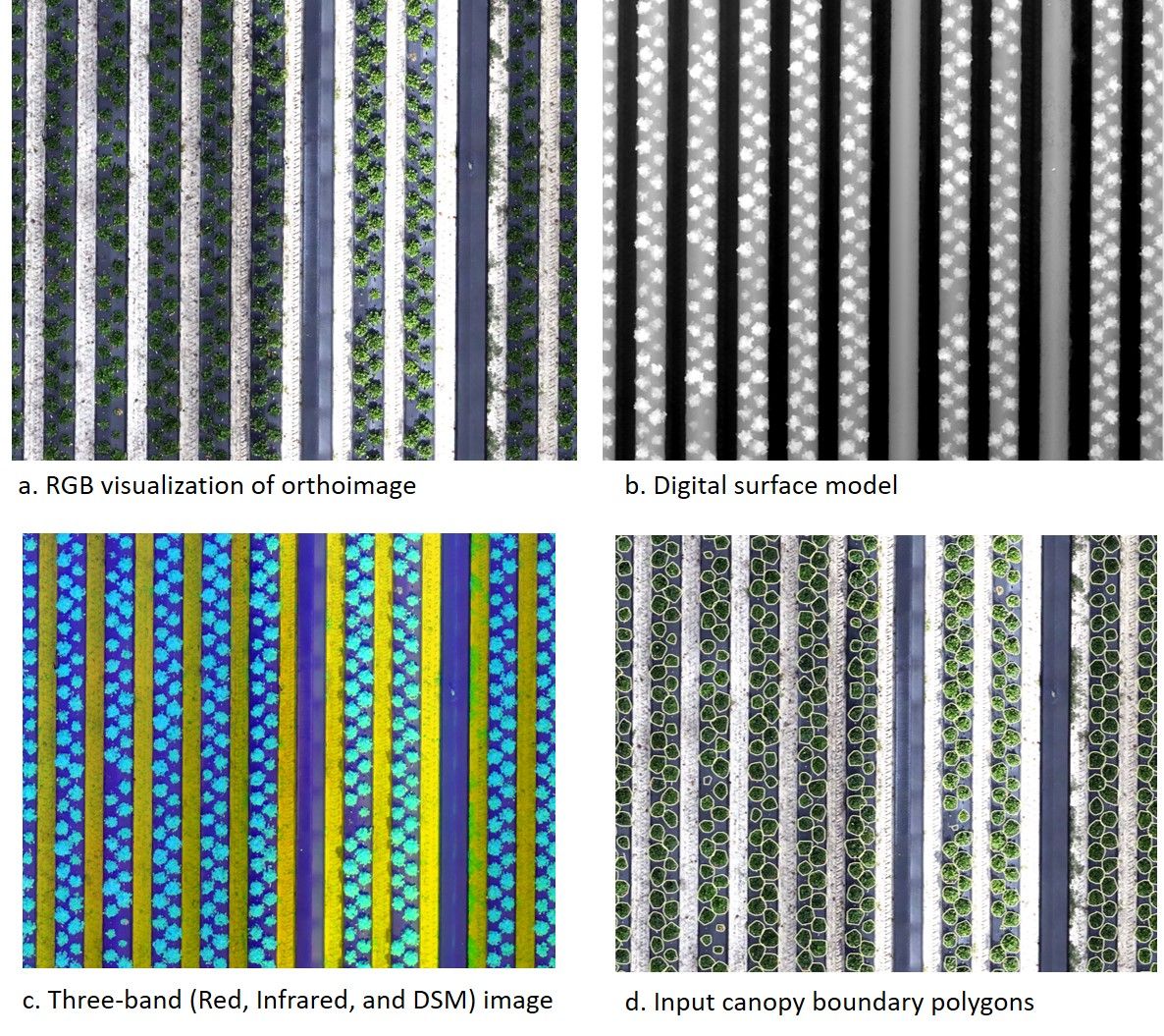
The dataset used in this study was captured at the UF/IFAS Gulf Coast Research and Education Center in Wimauma, Florida. High-resolution images were captured using two Nikon D300 cameras mounted about 4m above the strawberry beds on a platform towed by a tractor as explained in Abd-Elrahman et al. (2020). The images were pre-processed using the Agisoft Metashape software (https://www.agisoft.com/downloads/installer/) according to the procedures described by Abd-Elrahman et al. (2020) and Kakarla and Ampatzidis (2019). Image pre-processing resulted in 1-mm pixel ortho-rectified images (orthoimages) and 2mm pixel Digital Surface Model (DSM) (Figure 1 a and b). The Red and Infrared bands from the orthoimage were combined with the DSM to produce a three-band image used in canopy delineation. Selection of these bands was based on the research published by Guan et al. (2020) and Abd-Elrahman et al. (2020), who utilized these three bands successfully to delineate canopies using traditional geospatial analysis methods.
Credit: undefined
To train the Mask RCNN classifier, three images captured on multiple dates (12/10/2018, 01/31/2019, and 02/28/2019) and their canopy boundaries, shown in Figure 1 c and d, were used. The delineated boundaries were in a shapefile format. Each included a field called Class, where each canopy had a value of 1 in the attribute table. The total number of canopies used for training was 10,273. Another dataset used was used to demonstrate the Mask RCNN canopy detection and delineation using an image captured on 01/31/2019. This image was used to implement the trained Mask RCNN model to produce canopy boundaries. All datasets used in this demonstration are available to allow the user to experiment and follow along with the presented workflow.
2. ArcGIS Pro version 2.5 Software Preparation for Deep Learning Analysis
The following needs to be applied to set up the python environment for the deep learning algorithms. Different instructions for other versions of the software can be found in https://pro.arcgis.com/en/pro-app/latest/help/analysis/deep-learning/install-deep-learning-frameworks.htm.
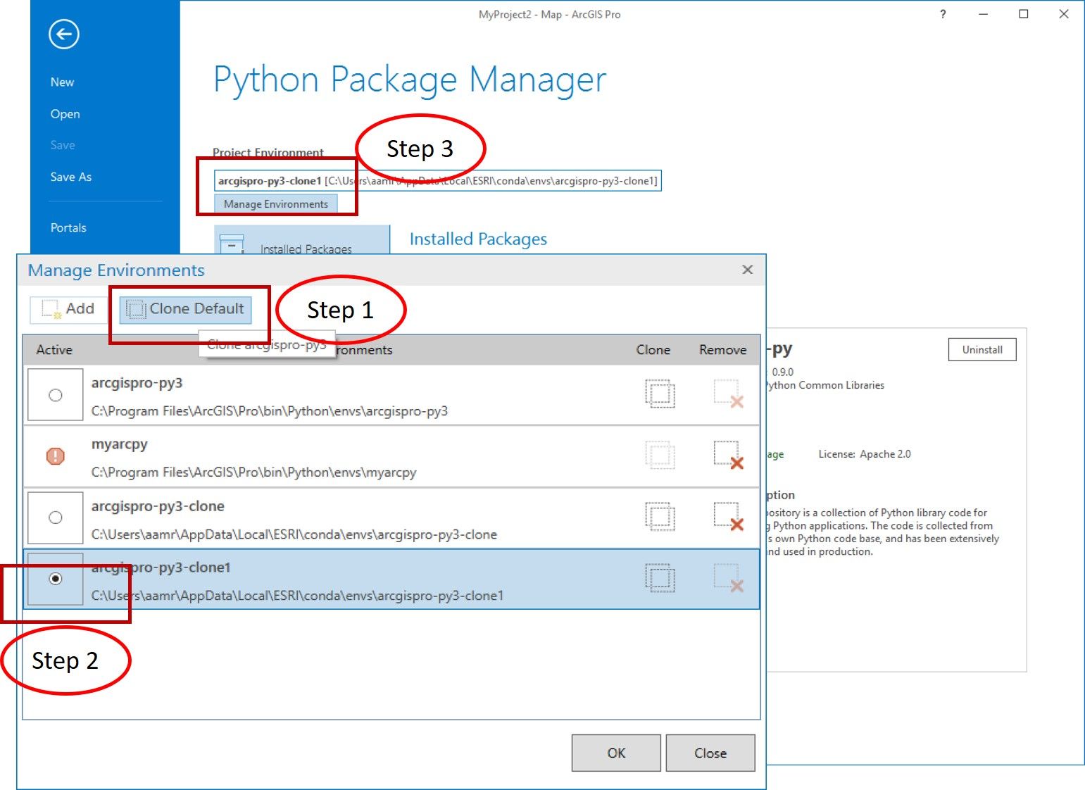
a. Clone and activate the Python Environment using the ArcGIS Pro interface. This process can also be done using the Python Command prompt. In the ArcGIS Pro interface, use: Project → Python → Manage Environment → Clone Default as shown in Figure 2. In the first step in the figure, the python environment is cloned. In the second step, the newly cloned environment is activated. Finally, in the third step, make sure the name of the cloned environment is shown in the marked box to verify the task is accomplished. Once this is verified, exit ArcGIS Pro.
Credit: undefined
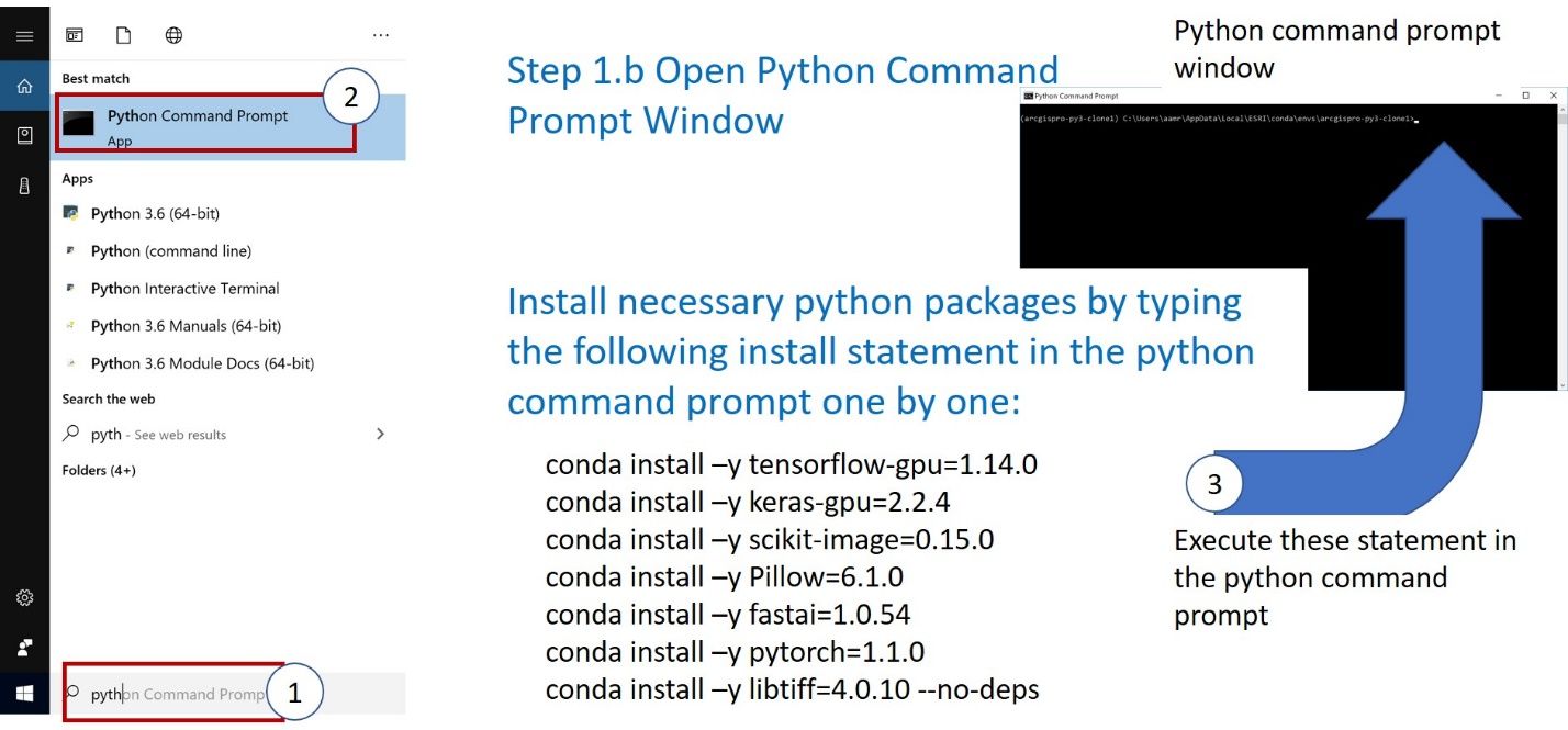
b. Open the Python Command Prompt Window, as shown in Figure 3 (steps 1 and 2), and install the necessary python packages by typing the following install statements in the python command prompt one by one (step 3):
CONDA INSTALL –Y TENSORFLOW-GPU=1.14.0
CONDA INSTALL –Y KERAS-GPU=2.2.4
CONDA INSTALL –Y SCIKIT-IMAGE=0.15.0
CONDA INSTALL –Y PILLOW=6.1.0
CONDA INSTALL –Y FASTAI=1.0.54
CONDA INSTALL –Y PYTORCH=1.1.0
CONDA INSTALL –Y LIBTIFF=4.0.10 --NO-DEPS
Credit: undefined
3. Extracting Training Dataset for Mask RCNN Analysis
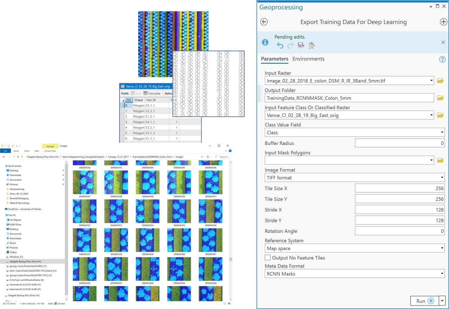
Three images captured on different dates and their delineated canopies were used to train the Mask RCNN model. Figure 4 (left) shows a snapshot of the ArcGIS Pro interface for the “Export Training Data for Deep Learning” tool. The input for the tool includes the image containing the canopies, the shapefile containing canopy boundaries, and the field name containing canopy class. If more than one input image is used, the tool should be repeated for each image and its corresponding canopy shapefile. All other parameters for the tool should remain the same. This tool creates chips of images from the input images with specified size (256x256) in this implementation. Each chip is accompanied by a corresponding chip of the classes (this example uses only one class in this implementation, which represents the canopies). The output is organized in a new folder, the name of which is specified in the tool. Figure 4 (right) shows a snapshot of some of the chips produced in one of the output folders containing training chips. Although this tool can run on the computer CPU, it executes much faster if the machine has a GPU. Setting up a GPU use is done through the Environment tab in the tool. The output of this process is used to train the model.
Credit: undefined
4. Mask RCNN Deep Learning Network Training
The most time-consuming process in deep learning is training, where numerous (hundreds to thousands to tens of millions) unknown parameters are determined through network training. Although the details of this process are outside the scope of this publication, it is mentioned here as a justification for the large size of the training dataset typically needed by convolutional neural networks, including Mask RCNN.
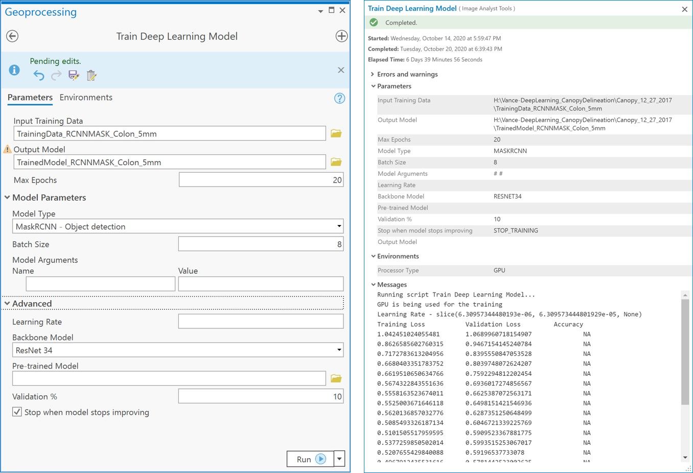
Network training is conducted using the “Train Deep Learning Network” tool in ArcGIS Pro as shown in Figure 5 (left). Tool input includes the name of the folder where the training data was extracted (i.e., the input of the previous step). Training specific information such as maximum number of epochs, batch size, type of deep learning architecture, and the percentage of data set aside for validation are also inputs in the tool. Network training is conducted iteratively. The whole training dataset is used in each training; however, due to limited computational capacity, only a subset of the training dataset is randomly selected and passed to the training algorithm. The “number of epochs” input parameter controls the maximum number of iterations the whole dataset will go through in the training process. The “batch size” input parameter specifies how many batches of the dataset will be selected randomly (without replacement) during each run and passed to the algorithm. This process continues until the whole dataset is consumed within each iteration. The number of batches is usually chosen according to the computational power of the machine. In our demonstration, we used the default (20) for the number of iterations and 8 for the number of batches. In the tool, we defined MaskRCNN -Object detection as the deep learning “Model Type” and ResNet34 as the “backbone model” (He et al. 2017). We also used 10% of the data for model “Validation %.” The trained model is stored in a new folder created by the user through the tool’s interface.
Credit: undefined
Figure 5 (right) shows the results of the Mask RCNN model training. The figure shows training and validation loss values. Those losses represent the difference between what the model produces and the given truth (correctly delineated canopies) for the training and validation datasets. The user should look for reduced training and validation loss and closer training and validation loss values for each epoch as the number of epochs increases. Training the model on CPU took more than 7 days on an Intel ®Xeon® CPU E3-1270 v5 @3.6 GHZ processor with 64 GB RAM computer. Training took about 6 hours when conducted using the GPU on a similar machine equipped with an NVIDIA Titan X Graphics card. Setting up GPU use is performed through the Environments tab in the tool. The output of model training is used in the next step to extract canopy boundaries from the images.
5. Canopy Delineation using the Mask RCNN Architecture
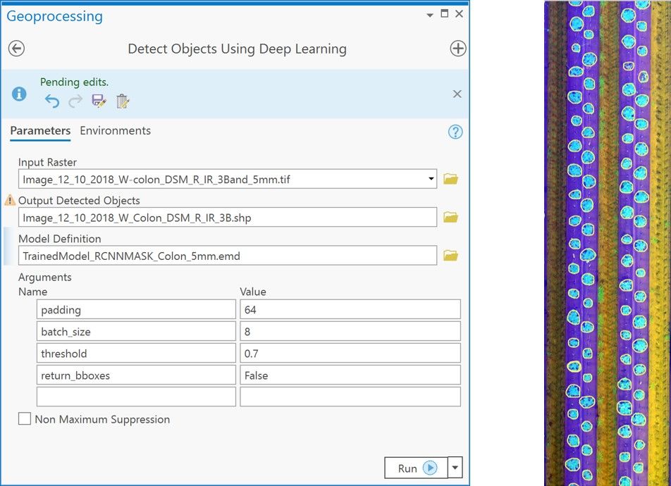
In this step, the trained model output from the previous step is used to create canopy boundaries from input images using the “DETECT OBJECTS USING DEEP LEARNING” ArcGIS Pro tool (Figure 6). The same type of images used to train the model must be used in this step. The folder containing the trained model information and the name of the output vector shapefile to store the delineated canopies are input parameters for the tool. Other input parameters include “BATCH SIZE” as described in the previous step. “PADDING” is a parameter indicating how many pixels the model should add to each image batch to avoid issues related to incomplete edge objects. The “THRESHOLD” parameter determines how much confidence in the delineated canopy we accept as a successful delineation. Only canopies with confidence higher than this threshold will be output. The last parameter shown in Figure 6 is the return boundary boxes (“RETURN_BBOXES”) flag, which indicates if a boundary box surrounding each canopy will also be returned. We set this parameter to FALSE because we are only interested in the polygon representing the canopy boundary. Again, there is a performance advantage for using a GPU to perform this step; however, a CPU-only machine, although slower, can also be used. Figure 6 shows the output of implementing the Mask RCNN network on a strawberry image captured on 01/31/2019 that is not part of the image used in training the model. Our visual inspection of the canopies indicates well-defined canopy boundaries that match non-deep-learning delineation results.
Credit: undefined
Discussion and Conclusion
This publication introduced a step-by-step deep learning implementation using widely available software packages. It builds on the knowledge acquired by the authors from developing geospatial analysis algorithms for canopy delineation. Although the demonstrated workflow was applied to strawberry canopies, we believe that this workflow can be applied to other crops once the model is trained using examples related to the target application. We used 10,273 canopies to train the model, but we believe that the model can be trained with fewer canopies and still produce reasonably reliable results.
Data Availability
Data used for this article is available to readers and can be found at the following link: https://drive.google.com/file/d/19_NXehuBrBdE64Ejkao-8eYminYZ9rOL.
Citations
Abd-Elrahman, A., Z. Guan, C. Dalid, V. Whitaker, K. Britt, B. Wilkinson, and A. Gonzalez. 2020. "Automated Canopy Delineation and Size Metrics Extraction for Strawberry Dry Weight Modeling Using Raster Analysis of High-Resolution Imagery." Remote Sensing 12 (21): 3632.
Ammirato, P., and A. C. Berg. 2019. "A Mask-RCNN Baseline for Probabilistic Object Detection." ArXiv Preprint.
Ding, P., Y. Zhang, P. Jia, and X. Chang. 2019. "A Comparison: Different DCNN Models for Intelligent Object Detection in Remote Sensing Images." Neural Processing Letters 49:1369–1379. https://doi.org/10.1007/s11063-018-9878-5
ESRI. 2019. Introduction to the ArcGIS Pro Image Analyst extension. Retrieved July 12, 2020, from https://pro.arcgis.com/en/pro-app/help/analysis/image-analyst/what-is-the-arcgis-pro-image-analyst-extension-.htm
Guan, Z., A. Abd-Elrahman, Z. Fan, V. M. Whitaker, and B. Wilkinson. 2020. "Modeling Strawberry Biomass and Leaf Area Using Object-Based Analysis of High-Resolution Images." ISPRS Journal of Photogrammetry and Remote Sensing 163:171–186. https://doi.org/10.1016/j.isprsjprs.2020.02.021
He, K., G. Gkioxari, P. Dollar, and R. Girshick. 2017. "Mask R-CNN." In Proceedings of the IEEE International Conference on Computer Vision (ICCV) (pp. 2961–2969).
Kakarla, S., and Y. Ampatzidis. 2019. "Postflight Data Processing Instructions on the Use of Unmanned Aerial Vehicles (UAVs) for Agricultural Applications." EDIS 6(6). https://doi.org/10.32473/edis-ae533-2019.
Kakarla, S., L. de Morais Nunes, and Y. Ampatzidis. 2019. "Preflight and Flight Instructions on the Use of Unmanned Aerial Vehicles (UAVs) for Agricultural Applications." EDIS 6(5). https://doi.org/10.32473/edis-ae535-2019.
Zhao, Z., P. Zheng, S. Xu, and W. Xi. 2019. "Object Detection with Deep Learning: A Review." IEEE Transactions on Neural Networks and Learning Systems 30 (11): 3212–3232. https://doi.org/10.1109/TNNLS.2018.2876865