Introduction
One of the main artificial intelligence (AI) techniques transforming the way we use remote sensing images in natural resource management applications is deep learning (Goodfellow et al. 2016). One of the outputs of applying deep learning on remote sensing images is classified images that are frequently used to study land cover changes and assist natural resources management efforts such as invasive plant detection and control. Although deep learning techniques have gained momentum in the field recently, the software skills needed to prepare the data, train the model, and implement the trained model in targeted applications present a major obstacle to wide-scale adoption and use of these techniques. This article demonstrates step-by-step implementation of the Unet deep learning semantic segmentation (image classification) network using the ArcGIS Pro v2.7 (Environmental Systems Research Institute 2019) software. This publication presents a guide to this technology to make it more widely accessible to GIS analysts, researchers, and graduate students working with remotely sensed data in the natural resource management field.
The demonstration in this publication uses images captured by Unmanned Aircraft System (UAS) of a wetland area in west central Florida. The dataset used deep learning implementations published in peer-reviewed manuscripts to facilitate result comparisons. The software interface of each step in the workflow is explained with input examples. The publication explains the major parameters needed for the Unet deep learning network data preparation, training, and image classification steps. Although we focus on image classification applications, the steps we demonstrate are generic and can be used as a framework for using deep learning networks in different natural resource management applications. We also discuss the achieved accuracy assessment of the resulting classification.
Background
Remote sensing image acquisition is becoming increasingly common. This comes with abundant unmanned aircraft systems (UAS; a.k.a. drones) use in natural resource management applications (Watts et al. 2008). Various recent EDIS publications illustrate how to perform post-flight analysis of drone images for agricultural applications (Kakarla and Ampatzidis 2019), emphasizing the increased need for this type of data analysis. However, tutorials on how to apply image classification techniques to automatically label each pixel with its land cover category are still lacking. This publication aims to provide simple techniques to apply state-of-the-art deep learning to analyze high-resolution images captured by drones and ground-based remote sensing platforms. The audience of this article is county and state geographic information system (GIS) analysts, researchers, and graduate students involved in remote sensing image analysis for natural resource management with basic GIS analysis experience. We demonstrate how to use the ESRI ArcGIS Pro software, one of the most widely used GIS software applications in the world. ArcGIS is widely used by federal and local government agencies including most government agencies in the state of Florida, including its university system. The dataset used in this article is the same dataset used by Liu et al. (2019), and the results obtained using the ArcGIS Pro software can be compared to the ones achieved by Liu and Abd-Elrahman (2018a; 2018b). The dataset is available as described in the “Data Availability” section at the end of this publication.
Recently, several deep convolutional neural network (DCNN) algorithms have gained momentum in different image analysis applications mainly due to their superior object detection, and semantic segmentation (classification) results and their ability to extract image features without human intervention. One of the main factors hindering DCNN from being implemented on a wider scale is the need for specific computer programming and operating system technical skills that are not common among natural resource and agricultural operation managers. The objective of this publication is to facilitate the use of deep learning image analysis through simplified step-by-step implementation using a broadly used software package. One of the most successful DCNN architectures is Unet (Ronneberger et al. 2015). The mathematical and technical aspects of Unet implementation are outside the scope of this publication and interested users can learn more about DCNN in general, and Unet specifically, by referring to many available resources (e.g., Zhao et al. 2019; Ding et al. 2019).
Dataset Preparation
The dataset used for this publication was captured in southern Florida, between Lake Okeechobee and Arcadia, Florida (Figure 1). The area used for the study is part of a large, 31,000-acre ranch with a diverse landscape composed of grass wetlands, tropical forage grass pastures, palmetto wet and dry praries, pine flatwoods, and interconnecting marsh areas. Typical vegetation includes cabbage palm, forage grasses, and live oak hammocks, which are usually located along the wet areas such as gullies, creeks, and other wetlands. Additionally, the area is infested with cogongrass (Imperata cylindrica) which is prevalent throughout the pasture areas. Cogongrass is a harmful, invasive species considered to be in the top ten most invasive weeds in the world. It is detrimental to the region because of its propensity to decrease native plant biodiversity, its destructiveness to native wildlife habitat, and its negative effect on real estate value. Additionally, cogongrass is extremely flammable, and large patches of it create a greatly increased hazard of fire. Effective identification of cogongrass cluster locations can help mitigation efforts of the US Army Corps of Engineers (USACE) and multiple other agencies engaged in routine monitoring and control operations to minimize the spread of this invasive grass in Florida.
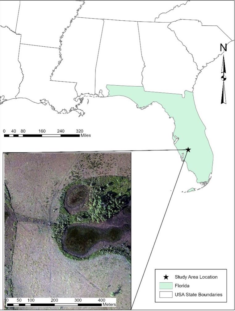
Credit: Amr Abd-Elrahman, Katie Britt, and Tao Liu
The aerial images used for this article were captured using a small, fixed-wing UAS by the USACE-Jacksonville District. The mission planning included an 83% forward overlap and a 50% sidelap for captured imagery from a Canon EOS REBEL SL1 digital camera. Image size was 3456 x 5184 pixels. An onboard navigational grade GPS receiver was used to synchronize the images with their locations. The photogrammetric solution involved five ground control points, with four near the corners and one near the center of the study site. The imagery captured by the Canon EOS REBEL SL1 was three-band, true color (RGB) imagery.
Liu and Abd-Elrahman (2018a; 2018b) created and used training polygons, which have been provided for use with this publication. Manual digitization of a large number of polygons was conducted with a high number for each class for both cogongrass and the seven other major land cover classes present in the study area and shown in Table 1 (Liu and Abd-Elrahman, 2018a). For this publication and the associated demonstration data provided, about 2,100 training polygons were included for the classes. Another 280 ground-truth points were also created and used to test the accuracy of the automated classification results demonstrated in the publication. The training data polygons and the accuracy ground truth points were prepared in standard shapefile GIS formats.
Table 1. Land cover classes in the study area.
Implementation Steps
- ArcGIS Pro Software preparation for deep learning analysis
The ESRI’s ArcGIS Pro v 2.7 (ESRI 2019) software was used to conduct the analysis. Uninstall any previous version of the ArcGIS Pro software and install the 2.7 version before completing the remaining steps. In order for ArcGIS Pro to use deep learning functionalities, the python environment for deep learning needs to be installed. Other software preparation techniques may be needed for newer versions of ArcGIS Pro. Please refer to “Install deep learning frameworks for ArcGIS” (https://pro.arcgis.com/en/pro-app/latest/help/analysis/deep-learning/install-deep-learning-frameworks.htm) for information on how to configure the ArcGIS Pro environment for the latest version. On the ArcGIS webpage, select the software version that suits the installed ArcGIS Pro version from the dropdown menu as shown in Figure 2.

Credit: Amr Abd-Elrahman, Katie Britt, and Tao Liu
a. Click the Deep Learning Libraries Installer for ArCGIS Pro link (shown in Figure 2). The link should take you to the github site containing the link to download the installation libraries. Download the installation package corresponding to the ArcGIS Pr v2.7 software as shown in Figure 3.
b. Make sure ArcGIS Pro is closed. Uncompress and install the downloaded installation package for ArcGIS Pro v2.7. This should install what is needed to run the deep learning tools.

Credit: Amr Abd-Elrahman, Katie Britt, and Tao Liu
- Training dataset extraction for Unet Analysis
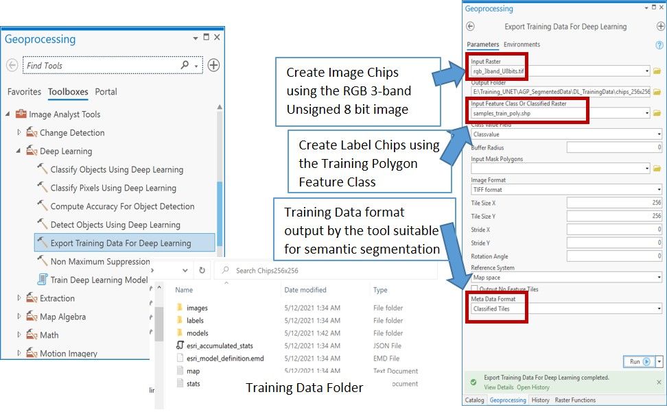
A three-band, RGB image (described in the Dataset Preparation section) was used to create the training dataset. In the ArcGIS Pro Geoprocessing toolbox, under Toolboxes, navigate to Image Analyst Tools → Export Training Data for Deep Learning (Figure 4). The Input Raster is the three-band, unsigned 8 bit raster. The Input Feature Class Or Classified Raster is the training data polygon shapefile (explained in the Dataset Preparation section) including many instances of each of the seven classes. The tool also asks to specify the Class Value Field, which indicates which attribute of the input feature class to use for the label for each training feature. The class label of training data polygon shapefile is represented by values from sequential numbers that start from 1 and end with the number of classes.
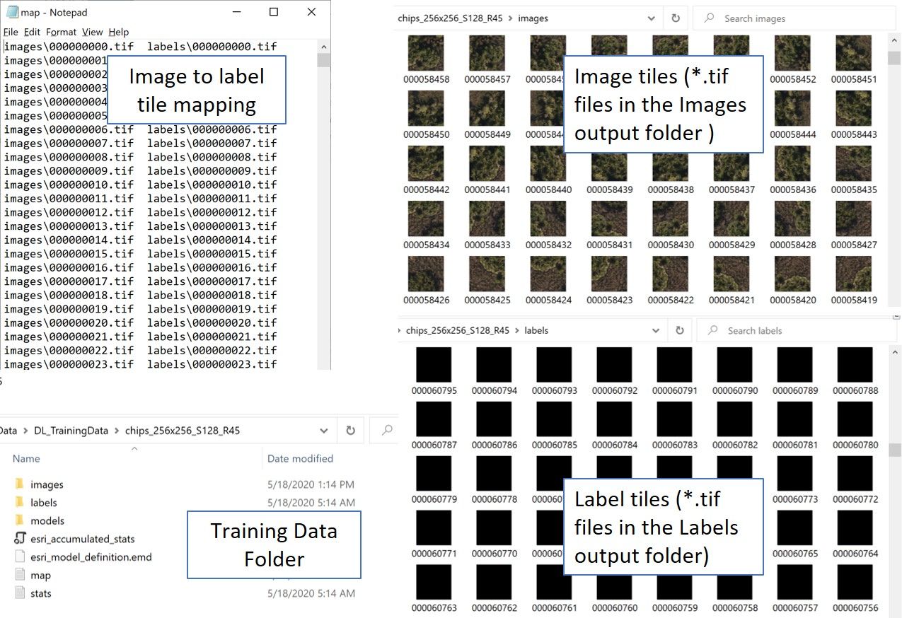
This tool creates pairs of tiles (sometimes called chips) from the input image and training polygon feature class with specified size (e.g. 256 x 256 in this implementation). The two tiles (called image and label tiles) correspond to the same location, with one being the RGB values of the input features and the second being a raster indicating the class number of the pixels based on the training polygons. In the folder you will find a text document that contains a list mapping each image tile to its corresponding labeled tile. The Stride X and Y of 128 indicates that 256 x 256 pixel tiles will be produced with 128 pixel shifts in the row and column directions so that each consecutive tile in the row or column directions will have 50% overlap. The Rotation parameter requests tiles to be produced at increments of 45-degree rotations. These last two parameters increase the size of the training dataset and lead to a significant increase in classification accuracy in our experiment.
To reduce the number of tiles produced that are not necessary to the training process, the Output No Feature Tiles box is left unselected, so that no tile will be produced if the training data does not use this location. The Meta Data Format of classified tiles is a generic choice for the results, but other dropdown choices include image detection or classification. The output tiles as well as other metadata (Figure 5) are created in a new folder specified in the tool.
Credit: Amr Abd-Elrahman, Katie Britt, and Tao Liu
Credit: Amr Abd-Elrahman, Katie Britt, and Tao Liu
2. Unet Deep Learning Network Training
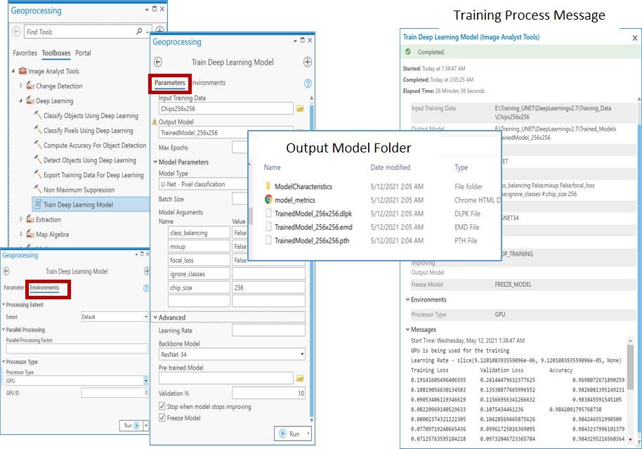
Once the training data is prepared, the next step is to use it to train the deep learning model. This is completed by navigating to the Geoprocessing toolbox → Toolboxes, and navigating to Image Analyst Tools → Deep Learning → Train Deep Learning Model. Figure 6 shows the Train Deep Learning Model tool input for both the Parameters and Environments tabs, as well as model information.
Credit: Amr Abd-Elrahman, Katie Britt, and Tao Liu
Under the Parameters tab, Input Training Data specifies the folder in which the training tiles were stored. The Output Model parameter specifies another folder name and location that will be created to store the model training results. The Validation % parameter specifies a percentage of the input training tiles selected randomly and set aside to validate the model at each iteration. We used 10% in this implementation.
In the Model Parameters section of the tool under Model Type, specify the U-Net – Pixel Classification type from the dropdown menu. Under Batch Size, specify how many tiles you will run in each iteration. This number can vary depending on the configuration of your computer given the computational requirements of the process. If you have the capability to run using GPU architecture, this will improve the computational strength for running the model, and you can specify this under the Environments tab in the Processor Type dropdown if available.
Back in the Parameters tab under Advanced, set the Backbone Model to ResNet 34. Check the box for Stop when model stops improving to direct the model to stop iterating when it is no longer strengthening as it continues.
When the tool is running, the message box will show the training loss, validation loss, and accuracy for each iteration. The training and validation losses are measures of the difference between model results and the training and validation data, respectively, at each iteration. The accuracy is a measure of how accurately the model is predicting the correct output based on the validation samples. Successful training is recognized by decreasing training and validation losses, training and validation losses that are approaching each other, and increasing validation accuracy. The output folder includes multiple files, but the EMD file is the file of the most significance to the user because it is the file that will be used in the semantic segmentation, or image classification step, next.
In developing this method, training the model using the computer central processing unit (CPU) was terminated after running for several days on a computer with an Intel®Xeon® CPU E3-1270 v5 @3.6 GHZ processor with 64 GB RAM. Training took 12 hours when conducted using the computer Graphics Processing Unit (GPU) on a similar machine equipped with an NVIDIA Titan X Graphics card, making it a more efficient choice.
3. Image Classification (semantic segmentation) using the Unet Architecture
In this step, the model that was created during the training process is passed to the classifier and applied to the entire study area. In the Geoprocessing toolbox, under Toolboxes, navigate to Image Analyst Tools → Deep Learning → Classify Pixels Using Deep Learning (Figure 7). To expedite the process, use a GPU if possible, specifying this under the Environments tab under Processor Type as mentioned in the previous step. In the Parameters tab, specify the input as the three-band, unsigned 8 bit TIF study area image under Input Raster. For the Output Classified Raster, specify the name and location of the output classified raster. Under Model Definition, specify the EMD file created in the previous step resulting from model training. In the Arguments section, set predict_background to false to cause the classification to predict class values. We set the batch_size argument to 8, which allows processing 8 tiles at a time. For the padding argument, you can select 16 or set it higher, at 56 or even 128. This parameter pads the tiles with the specified number of pixels to minimize issues related to edge effect between tiles. Figure 7 also shows the output classification using default symbology, which the user should adjust to use meaningful class numbers and labels.
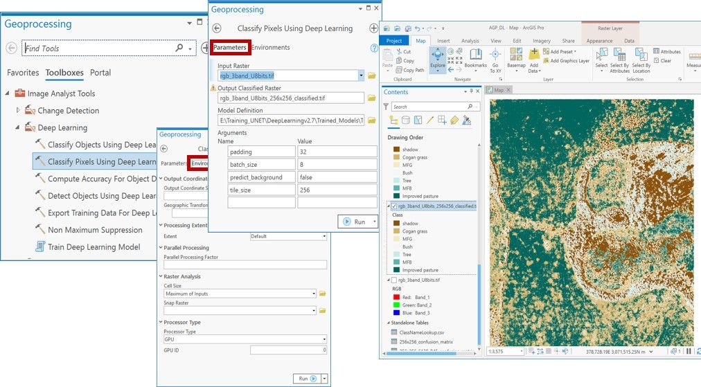
Credit: Amr Abd-Elrahman, Katie Britt, and Tao Liu
The output image was not of type integer, and the class numbers were shifted. We converted the image to a raster layer of type integer using the Int tool (integer tool) and applied the Reclassify tool to adjust the class numbers to match the training and testing data’s classes. In the Reclassify tool, enter the desired value to match the training and testing in the New column and specify the output raster if necessary.
4. Discussions and Accuracy Assessment
Accuracy Assessment was conducted using 280 randomly selected points (about 40 points per class) using the ArcGIS Pro Compute Confusion Matrix tool. The tool accepts a shape file with two fields named Classified and Ground truth to store the class resulting from the classification and corresponding ground truth class for each point, respectively. Figure 8 presents the confusion matrix (Jensen 2016) resulting from the accuracy assessment tool. The matrix cross references how many points of each ground truth class were found on the classification output classes (columns) and how many points in each classification output class belong to ground truth classes (rows). The number of points correctly identified is listed on the main diagonal of the matrix and the total number of correctly classified points divided by the total number of points represents the overall accuracy of the classification. The matrix also shows the Kappa Coefficient, another metric for classification accuracy (Jensen 2016). The overall accuracy assessment achieved in this demonstration was 82.5%, which matches the results obtained using more sophisticated analysis that used object-based framework, multi-view analysis, and full convolutional networks (Tao Liu and Abd-Elrahman 2018b; Tao Liu et al. 2019).
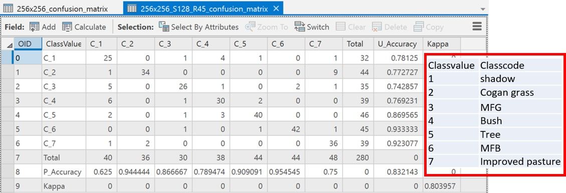
Credit: Amr Abd-Elrahman, Katie Britt, and Tao Liu
Conclusion
This publicationwas intended to provide simple, step-by-step instructions to use deep learning techniques to analyze high resolution imagery by performing classification on these data sets. This goal was achieved using the widelyused ESRI ArcGIS Pro software application. This work built on previous work bythe authors and provides a real world data set as an example for users to follow. Though the data set used here is specific to classification of invasive cogongrass, the workflow has wide ranging applications, and users will be able to apply this to many other agricultural and natural resource uses relevant to their individual fields.
Data Availability
Data used for this article are available to readers with an access request and can be found at the following link: https://drive.google.com/file/d/16zqxx6iW0RaMhY3SfVkYSt3Gj3mSnZOL/view?usp=sharing/.
Citations
Ding, Peng, Ye Zhang, Ping Jia, and Xu-ling Chang. 2019. “A Comparison: Different DCNN Models for Intelligent Object Detection in Remote Sensing Images.” Neural Processing Letters 49: 1369–79. https://doi.org/10.1007/s11063-018-9878-5.
Environmental Systems Research Institute. 2019. “ArcGIS Pro.”
Goodfellow, Ian, Yoshua Bengio, and Aaron Courville. 2016. Deep Learning. Cambridge: MIT press.
Jensen, John R. 2016. Introductory Digital Image Processing: A Remote Sensing Perspective. 4th ed. Pearson.
Kakarla, Sri, and Yiannis Ampatzidis. 2019. “Postflight Data Processing Instructions on the Use of Unmanned Aerial Vehicles (UAVs) for Agricultural Applications.” EDIS 6 (6). https://doi.org/10.32473/edis-ae533-2019.
Liu, T., and A. Abd-Elrahman. 2018. “An Object-Based Image Analysis Method for Enhancing Classification of Land Covers Using Fully Convolutional Networks and Multi-View Images of Small Unmanned Aerial System.” Remote Sensing 10 (3): 457.
Liu, Tao, and Amr Abd-Elrahman. 2018. “Deep Convolutional Neural Network Training Enrichment Using Multi-View Object-Based Analysis of Unmanned Aerial Systems Imagery for Wetlands Classification.” ISPRS Journal of Photogrammetry and Remote Sensing 139 (May): 154–70. https://doi.org/10.1016/j.isprsjprs.2018.03.006.
Liu, Tao, Amr Abd-Elrahman, Bon Dewitt, Scot Smith, Jon Morton, and Victor L. Wilhelm. 2019. “Evaluating the Potential of Multi-View Data Extraction from Small Unmanned Aerial Systems (UASs) for Object-Based Classification for Wetland Land Covers.” GIScience & Remote Sensing 56 (1): 130–59. https://doi.org/10.1080/15481603.2018.1495395.
Ronneberger, Olaf, Philipp Fischer, and Thomas Brox. 2015. “U-Net: Convolutional Networks for Biomedical Image Segmentation.” In International Conference on Medical Image Computing and Computer-Assisted Intervention, edited by N. Navab, J. Hornegger, W. Wells, and A. Frangi, 234–41. Springer, Cham. https://doi.org/10.1007/978-3-319-24574-4_28.
Watts, A. C., W .S. Bowman, A. Abd-Elrahman, A. Mohamed, B. Wilkinson, J. Perry, Y. Kaddoura, and K. Lee. 2008. “Unmanned Aircraft Systems (UASs) for Ecological Research and Natural-Resource Monitoring (Florida).” Ecological Restoration 26 (1): 13–14. http://er.uwpress.org/content/26/1/13.short.
Zhao, Z., P. Zheng, S. Xu, and Wu. Xi. 2019. “Object Detection with Deep Learning: A Review.” IEEE Transactions on Neural Networks and Learning Systems 30 (11): 3212–32. https://doi.org/10.1109/TNNLS.2018.2876865.